Introduction
Hands-On LLM Implementation
Build everything from scratch. Ship to production.
A practical, implementation-first guide to training and deploying large language models
Who this book is for
You already understand the theory. You want to build the thing.
Every chapter here is backed by a working project in the companion repository,
llm-from-scratch. The
tokenizer, attention, training loop, and contrastive objective are all written
from scratch, with the original research papers cited in the source code.
Across the book we assemble one pipeline: tokenization, pre-training, fine-tuning, optimization, and production deployment.
What the first four chapters cover
- Character-Level GPT. Attention, transformer blocks, and a training loop, small enough to understand every line.
- The BPE Tokenizer. Subword tokenization, the same method GPT-2 and GPT-3 use.
- Contextual Embeddings. A BERT-style bidirectional encoder trained with masked language modeling.
- SimCSE. Contrastive learning that turns the encoder into a sentence-embedding model, where dropout is the only data augmentation.
Later phases (fine-tuning, inference optimization, quantization, parallelism, deployment) follow the same pattern: implement it, measure it against the paper, ship it.
How this differs from a tutorial
- The documentation is paper-first. Every module’s docstrings quote the paper
it implements (
PAPER:,PAPER CONTEXT:,INTUITION:,IMPLEMENTATION:,WHY:), so the code and the literature don’t drift apart. - The results are measured. Each chapter ends with numbers from real runs on a single consumer GPU (an 8 GB RTX 3050), not the ones we wish we’d got.
- Nothing is a black box. If a component appears in the code, the book explains why it was designed that way.
Conventions used in this book
- Code blocks reference files in the repository, e.g.
phase1_foundation/project3b_simcse/model.py - All commands run from the repository root with
uv run python ... - Citations like (Gao, Yao & Chen, 2021) refer to the papers listed at the end of each chapter.
Start with Getting Set Up, then head to Chapter 1.
Getting Set Up
Hardware
Everything in Part I was built and trained on a single consumer GPU:
| Requirement | Details |
|---|---|
| GPU | CUDA-capable; 8 GB VRAM recommended (all runs here used an RTX 3050 8 GB) |
| Python | 3.10–3.13 |
| Env manager | uv |
| Knowledge | Neural networks & attention (theory only; we implement the rest) |
Installation
# Clone
git clone git@github.com:abubakarsiddik31/llm-from-scratch.git
cd llm-from-scratch

# Install all dependencies (PyTorch CUDA wheels are pre-configured)
uv sync --group all
GPU notes
The repository’s pyproject.toml pins PyTorch to the CUDA 12.8 wheel
index, so uv sync installs a GPU build by default:
[tool.uv.sources]
torch = [{ index = "pytorch-cu128" }]

[[tool.uv.index]]
name = "pytorch-cu128"
url = "https://download.pytorch.org/whl/cu128"
explicit = true
On a CPU-only machine, remove that block to fall back to CPU builds. Verify your setup:
uv run python -c "import torch; print(torch.cuda.is_available(), torch.cuda.get_device_name(0))"
# True NVIDIA GeForce RTX 3050
Tip: do not keep the repository inside a cloud-synced folder (OneDrive, Dropbox). Checkpoint writes during training are large and frequent; sync clients cause lock conflicts and slow I/O. Keep it on a local disk.
Running the projects
All commands run from the repository root via uv run:
# Chapter 1 — train character-level GPT, then generate
uv run python phase1_foundation/project1_minimal_gpt/train.py
uv run python phase1_foundation/project1_minimal_gpt/generate.py --prompt "ROMEO:" --interactive

# Chapter 2 — download data, train tokenizer, test it
uv run python phase1_foundation/project2_tokenizer/download_data.py --size small
uv run python phase1_foundation/project2_tokenizer/train_tokenizer.py --vocab_size 5000
uv run python phase1_foundation/project2_tokenizer/test_tokenizer.py --interactive

# Chapter 3 — BERT-style MLM/NSP pre-training
uv run python phase1_foundation/project3_contextual_embeddings/download_data.py --size small
uv run python phase1_foundation/project3_contextual_embeddings/train.py

# Chapter 4 — SimCSE
uv run python phase1_foundation/project3b_simcse/download_data.py
uv run python phase1_foundation/project3b_simcse/test_model.py   # sanity tests
uv run python phase1_foundation/project3b_simcse/train.py
uv run python phase1_foundation/project3b_simcse/evaluate.py
Repository layout
llm-from-scratch/
├── phase1_foundation/
│   ├── project1_minimal_gpt/           # Chapter 1
│   ├── project2_tokenizer/             # Chapter 2
│   ├── project3_contextual_embeddings/ # Chapter 3
│   └── project3b_simcse/               # Chapter 4
├── data/            # gitignored: downloaded corpora
└── checkpoints/     # gitignored: trained models
Each project follows the same structure: config.py (hyperparameters with
paper references), the core implementation, a training script, a test script,
and a data downloader. Checkpoints are .pt/.pkl files with model state,
optimizer state, and metrics.
Character-Level GPT
Project source:
phase1_foundation/project1_minimal_gpt/Papers: “Attention Is All You Need” (Vaswani et al., 2017) · “Improving Language Understanding by Generative Pre-Training” (GPT-1, 2018) · “Language Models are Unsupervised Multitask Learners” (GPT-2, 2019)
Objective
Build a GPT model from scratch and train it on Shakespeare. By the end you will have implemented, without a library doing the work for you:
- Self-attention, the core mechanism of the transformer
- Multi-head attention: parallel heads learning different patterns
- The transformer block: attention and a feed-forward network joined by residuals
- Positional embeddings, so the model has a sense of sequence order
- The training loop: loss, backpropagation, optimization
- Text generation with temperature and top-k sampling
Why start at character level?
| Character-level | Word/subword level | |
|---|---|---|
| Tokenization | Trivial (each character is a token) | Needs BPE (Chapter 2) |
| Vocabulary | ~65 tokens | 50,000+ |
| Time to first result | Minutes | Hours |
| Debugging | You can visually inspect everything | Harder |
The model is small, roughly 10M parameters, and the dataset is about a million characters, so training finishes in under an hour on a consumer GPU. That is fast enough to iterate on an idea instead of waiting on it.
Architecture
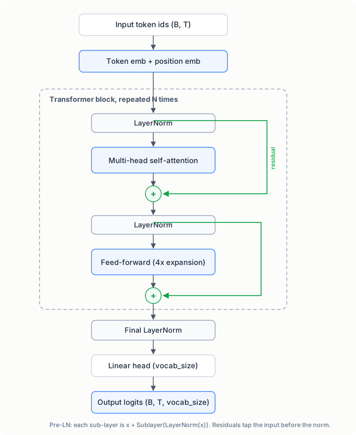
Note the pre-LN arrangement: LayerNorm sits before each sublayer. That is the GPT-2 style, and it trains more stably than the original post-LN design.
The core ideas
Self-attention
Every token asks two questions: what am I looking for? (its query) and what do I contain? (its key and value).
For each token position:
- Query (Q): "What am I looking for?"
- Key (K):   "What do I contain?"
- Value (V): "What information do I provide?"

Attention = softmax(Q × Kᵀ / √d_k) × V
The √d_k scaling keeps softmax inputs in a healthy range. Without it, the
dot products grow with dimension and softmax saturates.
Causal masking
GPT generates text left to right, so position t may only attend to positions up to and including t. A triangular mask enforces this before the softmax:
- Position 1 sees: [1]
- Position 2 sees: [1, 2]
- Position T sees: [1, 2, ..., T]
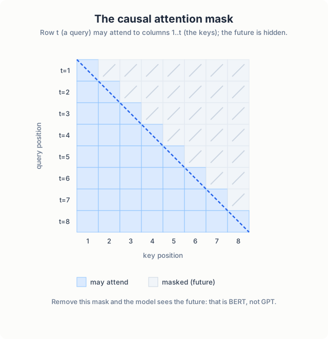
Remove that one mask and the model can see the future. This is the real difference between GPT (generation) and BERT (understanding): Chapter 3 removes it.
Multi-head attention
Instead of one attention computation, we run several in parallel on smaller projected subspaces. Different heads specialize: one might track syntax, another pronoun references. Their outputs are concatenated and projected back.
Residuals + LayerNorm
Each sub-layer is wrapped as x = x + Sublayer(LayerNorm(x)). The residual
gives gradients a highway through the network; the normalization stabilizes
activation scales across depth.
The code
Everything in this section is the actual repository code. The files in
phase1_foundation/project1_minimal_gpt/
carry long commentary docstrings alongside every line; what follows is the
same code with that commentary trimmed so the page stays readable. Excerpts
are condensed and lightly reformatted; the logic matches the repository.
The attention module
class CausalSelfAttention(nn.Module):
    # PAPER: "Attention Is All You Need", Vaswani et al. (2017), Sections 3.2.1-3.2.2

    def __init__(self, config):
        super().__init__()
        assert config.N_EMBD % config.N_HEAD == 0      # d_model must split evenly across heads
        self.n_head = config.N_HEAD
        self.head_size = config.N_EMBD // config.N_HEAD  # d_k = d_model / h

        # one projection produces Q, K and V together
        self.c_attn = nn.Linear(config.N_EMBD, 3 * config.N_EMBD, bias=False)
        # the W^O output projection from the multi-head formula
        self.c_proj = nn.Linear(config.N_EMBD, config.N_EMBD, bias=False)
        self.attn_dropout = nn.Dropout(config.DROPOUT)
        self.resid_dropout = nn.Dropout(config.DROPOUT)

        # lower-triangular ones: 1 = may attend, 0 = masked out
        self.register_buffer(
            "mask", torch.tril(torch.ones(config.BLOCK_SIZE, config.BLOCK_SIZE))
        )
Three decisions trace directly to the papers. The paper’s multi-head
formula needs d_k = d_model / h, which is why the divisibility assertion
is the first line of the module. The paper projects queries, keys and
values with separate matrices; doing it in one nn.Linear and splitting is
mathematically identical and one matrix multiply cheaper, and both GPT-1
and GPT-2 do the same. And the mask is a register_buffer, not a
parameter: it must be saved with the model and move to the GPU with it,
but no optimizer should ever touch it.
The forward pass is where the paper’s equation (1) lives:
    def forward(self, x):
        B, T, C = x.size()

        # (B, T, C) -> three tensors of (B, T, C): query, key, value
        q, k, v = self.c_attn(x).split(self.n_embd, dim=2)

        # split d_model across heads: (B, T, C) -> (B, n_head, T, head_size)
        k = k.view(B, T, self.n_head, self.head_size).transpose(1, 2)
        q = q.view(B, T, self.n_head, self.head_size).transpose(1, 2)
        v = v.view(B, T, self.n_head, self.head_size).transpose(1, 2)

        # softmax(Q K^T / sqrt(d_k))  -- paper equation (1)
        att = (q @ k.transpose(-2, -1)) * (self.head_size ** -0.5)

        # the causal mask: future positions get -inf, so softmax gives them 0
        att = att.masked_fill(self.mask[:T, :T] == 0, float("-inf"))

        att = F.softmax(att, dim=-1)
        att = self.attn_dropout(att)

        y = att @ v                                        # weighted sum of values
        y = y.transpose(1, 2).contiguous().view(B, T, C)   # concatenate heads
        y = self.resid_dropout(self.c_proj(y))             # the W^O projection
        return y
Four lines carry the whole mechanism. q @ k.transpose(-2, -1) turns
every token’s query against every token’s key into a (T, T) score
matrix. Multiplying by head_size ** -0.5 is the 1/√d_k scaling: without
it, dot products grow with dimension, softmax saturates, and gradients
vanish. masked_fill stamps -inf into every position that looks into the
future, so that after the softmax those entries are exactly zero. And
att @ v is each position collecting a weighted average of the values.
The reshape before and after only exist to give each of the n_head
heads its own head_size-dimensional slice to work on; the paper’s
“concatenate the heads” is the transpose(...).view(...) line.
The module returns a tensor with the same shape it received. That is
deliberate and it is what makes the residual connections in the next
section possible: x = x + Attention(x) only type-checks if attention
preserves shape.
The block and the feed-forward network
class FeedForward(nn.Module):
    # PAPER: "Attention Is All You Need", Section 3.3; 4x expansion follows GPT-2
    def __init__(self, config):
        super().__init__()
        self.net = nn.Sequential(
            nn.Linear(config.N_EMBD, 4 * config.N_EMBD),
            nn.ReLU(),
            nn.Linear(4 * config.N_EMBD, config.N_EMBD),
            nn.Dropout(config.DROPOUT),
        )

    def forward(self, x):
        return self.net(x)


class TransformerBlock(nn.Module):
    # PAPER: "Attention Is All You Need", Section 3.1; pre-LN ordering from GPT-2

    def __init__(self, config):
        super().__init__()
        self.attn = CausalSelfAttention(config)
        self.ffwd = FeedForward(config)
        self.ln1 = nn.LayerNorm(config.N_EMBD)
        self.ln2 = nn.LayerNorm(config.N_EMBD)

    def forward(self, x):
        x = x + self.attn(self.ln1(x))   # residual, LayerNorm applied first
        x = x + self.ffwd(self.ln2(x))   # residual, LayerNorm applied first
        return x
The forward pass is four lines, and the order of operations in them is the
single most consequential design choice in the file. The original
transformer normalized after each sub-layer
(x = LayerNorm(x + Sublayer(x)), “post-LN”). GPT-2 moved the norm
before the sub-layer (x = x + Sublayer(LayerNorm(x)), “pre-LN”), which
leaves a clean identity path from output back to input through the
residuals and trains noticeably more stably as depth grows. Every modern
decoder stacks blocks this way. The + is the residual: it gives gradients
a highway, and it means each sub-layer only has to learn a correction to
the signal rather than reproduce it.
The full model
class GPT(nn.Module):
    # PAPERS: GPT-1, Radford et al. (2018); GPT-2, Radford et al. (2019)

    def __init__(self, config):
        super().__init__()
        self.transformer = nn.ModuleDict(
            dict(
                wte=nn.Embedding(config.VOCAB_SIZE, config.N_EMBD),  # tokens
                wpe=nn.Embedding(config.BLOCK_SIZE, config.N_EMBD),  # positions
                drop=nn.Dropout(config.DROPOUT),
            )
        )
        blocks = [TransformerBlock(config) for _ in range(config.N_LAYER)]
        self.transformer.blocks = nn.ModuleList(blocks)
        self.transformer.ln_f = nn.LayerNorm(config.N_EMBD)
        self.lm_head = nn.Linear(config.N_EMBD, config.VOCAB_SIZE, bias=False)

    def forward(self, idx, targets=None):
        device = idx.device
        B, T = idx.shape

        tok_emb = self.transformer.wte(idx)   # (B, T, C): what each token is
        pos = torch.arange(0, T, dtype=torch.long, device=device)
        pos_emb = self.transformer.wpe(pos)   # (T, C): where each token sits
        x = self.transformer.drop(tok_emb + pos_emb)

        for block in self.transformer.blocks:
            x = block(x)

        x = self.transformer.ln_f(x)
        logits = self.lm_head(x)              # (B, T, vocab_size)

        loss = None
        if targets is not None:
            loss = F.cross_entropy(
                logits.view(-1, logits.size(-1)),
                targets.view(-1),
                ignore_index=-1,
            )
        return logits, loss
Both embeddings are learned lookup tables. The original transformer
computed positions with fixed sine/cosine patterns; GPT-1 switched to
learned position embeddings, which is simpler and works just as well at
fixed context length. Note the two embeddings are added, not
concatenated, so “cat” at position 0 and “cat” at position 5 get different
input vectors while the dimensionality stays at n_embd.
The loss line does next-token prediction over the whole sequence at once.
Because of the causal mask, position t’s logits were computed without
ever seeing token t+1, so the same forward pass yields T honest
training examples. logits.view(-1, vocab_size) flattens batch and time
into one list of predictions, and cross-entropy does the rest.
Generation
    @torch.no_grad()
    def generate(self, idx, max_new_tokens, temperature=1.0, top_k=None):
        for _ in range(max_new_tokens):
            idx_crop = (
                idx if idx.size(1) <= self.config.BLOCK_SIZE
                else idx[:, -self.config.BLOCK_SIZE :]
            )
            logits, _ = self(idx_crop)
            logits = logits[:, -1, :] / temperature   # only the last position matters

            if top_k is not None:
                v, _ = torch.topk(logits, min(top_k, logits.size(-1)))
                logits[logits < v[:, [-1]]] = -float("Inf")

            probs = F.softmax(logits, dim=-1)
            idx_next = torch.multinomial(probs, num_samples=1)
            idx = torch.cat((idx, idx_next), dim=1)
        return idx
Two details are easy to miss. The crop at the top only works because the
attention is causal: the next-token prediction depends on the last
BLOCK_SIZE tokens and nothing earlier, so discarding the prefix is free.
And the top-k trick is two lines: find the k-th largest logit, then set
everything below it to -inf, which removes the tail of implausible
tokens from the sampling distribution without changing the ranking of the
survivors.
Training
uv run python phase1_foundation/project1_minimal_gpt/train.py
Typical trajectory on Shakespeare:
step 0:    val loss 4.50   (random predictions)
step 500:  val loss 2.80   (learning patterns)
step 1000: val loss 2.20   (basic structure)
step 2000: val loss 1.90   (coherent text)
step 5000: val loss 1.60   (Shakespeare-like)
Expect a validation loss of 1.5–1.8 after roughly 30 minutes to 2 hours on a GPU.
Generation
# Single prompt
uv run python phase1_foundation/project1_minimal_gpt/generate.py \
    --prompt "ROMEO:" --temperature 0.8 --top_k 50

# Interactive mode (supports `temp <x>`, `topk <x>`, `clear`)
uv run python phase1_foundation/project1_minimal_gpt/generate.py --interactive
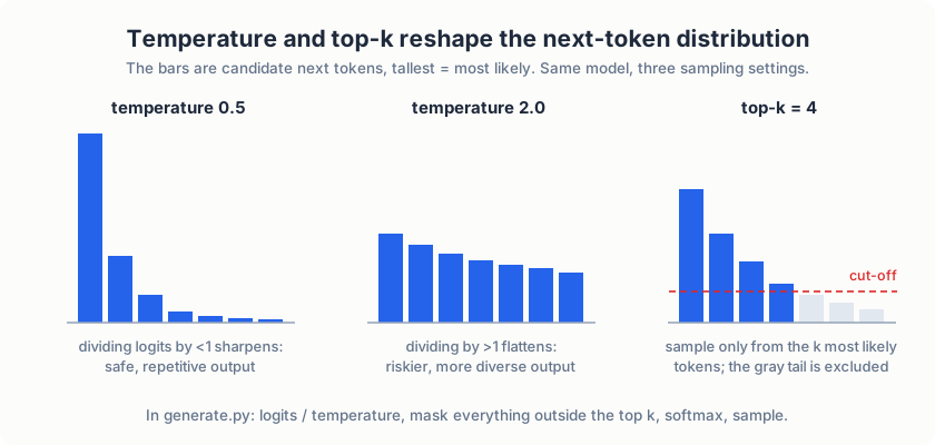
Temperature divides the logits before softmax: below 1 sharpens the distribution (safer, more repetitive), above 1 flattens it (riskier, more diverse). Top-k restricts sampling to the k most likely tokens, cutting off the long tail of implausible continuations.
Code tour
| File | What to read |
|---|---|
model.py | CausalSelfAttention, the transformer block, the full GPT class |
train.py | Batching, loss, the training loop, checkpointing |
generate.py | Autoregressive decoding, temperature/top-k |
config.py | Every hyperparameter, documented |
Exercises
- Set the causal mask to identity (no masking) and watch generation collapse into nonsense: the model now sees the future.
- Change
N_HEADto 1. How does the loss curve change? - Set
temperatureto 0.1 and to 2.0, and compare output quality.
What’s next
The model understands characters, not words. Chapter 2 builds the subword tokenizer that real LLMs use.
The BPE Tokenizer
Project source:
phase1_foundation/project2_tokenizer/Papers: “Byte-Pair Encoding: Subword-Based Machine Translation” (Sennrich, Haddow & Birch, 2016) · “A New Algorithm for Data Compression” (Gage, 1994 — original BPE) · WikiText (Merity et al., 2016)
Why subwords?
Chapter 1’s model saw characters: no unknown tokens, but every word cost many positions of context. Word-level models waste the opposite way: huge vocabularies and no way to handle unseen words. Byte-Pair Encoding sits in between, and it is the tokenization used by GPT-2, GPT-3, and most modern LLMs.
| Approach | Example | Pros | Cons |
|---|---|---|---|
| Character | "hello" → h e l l o | No unknowns, tiny vocab | Very long sequences |
| Word | "hello" → hello | Short sequences | Huge vocab, unknowns |
| BPE | "hello" → hello, "hells" → hell · s | Balanced, handles OOV | Moderate vocab |
Key properties:
- Handles OOV:
"unfriendliness"→un · friend · li · ness - Efficient: frequent words become single tokens
- Compositional: subwords recur across related words (
help,help · ing,help · ful) - No unknowns: worst case, every text degrades to characters
The training algorithm
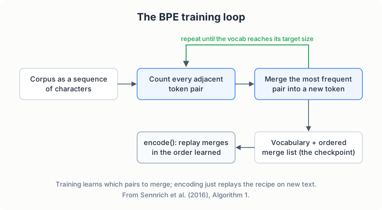
From Sennrich et al. (2016), Algorithm 1:
1. Initialize the vocabulary with all unique characters
2. Repeat until the target vocabulary size is reached:
   a. Count the frequency of every adjacent token pair
   b. Find the most frequent pair
   c. Merge it into a new token
   d. Apply the merge everywhere in the corpus
Worked example on "hug hug pug hug pug":
| Step | Operation | Vocabulary |
|---|---|---|
| Initial | characters | {h, u, g, p, ␣} |
| 1 | merge u+g → ug | {h, u, g, p, ␣, ug} |
| 2 | merge h+ug → hug | {h, u, g, p, ␣, ug, hug} |
| 3 | merge p+ug → pug | {h, u, g, p, ␣, ug, hug, pug} |
After training, encoding is greedy longest-match-first: apply the learned merges in the order they were learned.
Learned merges: [('e','r'), ('er','t'), ('ert','a')]
Text: "erter"
Step 1: ['e','r','t','e','r']
Step 2: ['er','t','e','r']      (apply 'e'+'r')
Step 3: ['ert','e','r']         (apply 'er'+'t')
Step 4: ['ert','er']            (apply 'e'+'r')
Scaling the training loop
The naive implementation recounts every adjacent pair across the entire corpus on every merge, which is O(corpus length) per merge. On an 11 MB WikiText corpus with a 5,000-token vocabulary that measured ~4.7 s/merge: a 5-hour run.
The fix in this repository is to represent the corpus as distinct words
with multiplicities (a Counter), so each merge iterates over ~50k unique
words instead of millions of characters, weighting pair counts by word
frequency. Merges still cross the word/space boundary because every word
carries a trailing space into training (so tokens like "the " are
learnable).
The result: about 5.8 merges per second, the same run in roughly 12 minutes, and an identical vocabulary. That’s a ~50× speedup for a representation change, not an algorithm change.
The code
As in Chapter 1, what follows is the repository’s code
(tokenizer.py)
with the commentary docstrings trimmed. Excerpts are condensed and lightly
reformatted; the logic matches the repository.
The training loop
class BPETokenizer:
    # PAPER: "Byte-Pair Encoding: Subword-Based Machine Translation",
    #        Sennrich et al. (2016), Algorithm 1

    def train(self, text, vocab_size, min_frequency):
        # 1. seed the vocabulary with every character in the corpus
        chars = sorted(list(set(text)))
        for char in chars:
            if char not in self.vocab:
                new_id = len(self.vocab)
                self.vocab[char] = new_id
                self.inverse_vocab[new_id] = char

        # 2. represent the corpus as distinct words with multiplicities
        normalized = " ".join(text.split())
        raw_words = normalized.split(" ")
        word_counts = Counter()
        for w in raw_words[:-1]:
            if w:
                word_counts[w + " "] += 1    # trailing space: word boundaries stay mergeable
        if raw_words and raw_words[-1]:
            word_counts[raw_words[-1]] += 1
        words = [list(w) for w in word_counts.keys()]

        # 3. the merge loop
        num_merges = vocab_size - len(config.SPECIAL_TOKENS) - len(chars)
        for merge_idx in range(num_merges):
            pair_counts = self._get_pair_counts(words, counts=list(word_counts.values()))
            if not pair_counts:
                break
            best_pair = max(pair_counts, key=pair_counts.get)
            if pair_counts[best_pair] < min_frequency:
                break

            new_token = best_pair[0] + best_pair[1]
            new_id = len(self.vocab)
            self.vocab[new_token] = new_id
            self.inverse_vocab[new_id] = new_token
            self.merges.append(best_pair)    # order matters: encode() replays it

            words = self._apply_merge(words, best_pair)
The trailing-space line deserves a pause. WikiText-2 is 11 MB of words
separated by whitespace, and BPE counts adjacent pairs; if words were
treated as isolated islands, the token the could never absorb the space
after it and real tokenizers’ the-with-trailing-space token would be
unlearnable. Appending the space to every word except the last keeps the
corpus equivalent to one long sequence, minus merges across newlines.
self.merges.append(best_pair) looks incidental and is not: encoding a
new string replays the merge list in exactly the order it was learned.
The same pair (a, b) merged early is a different operation than merged
late, because what a and b are depends on every merge before it.
Counting and applying a merge
    def _get_pair_counts(self, words, counts=None):
        # "Count the frequency of each adjacent pair" (Algorithm 1, step 2a)
        if counts is None:
            counts = [1] * len(words)
        pair_counts = Counter()
        for word, count in zip(words, counts):
            for i in range(len(word) - 1):
                pair = (word[i], word[i + 1])
                pair_counts[pair] += count
        return pair_counts

    def _apply_merge(self, words, pair):
        new_token = pair[0] + pair[1]
        new_words = []
        for word in words:
            new_word = []
            i = 0
            while i < len(word):
                if i < len(word) - 1 and word[i] == pair[0] and word[i + 1] == pair[1]:
                    new_word.append(new_token)
                    i += 2                   # both symbols consumed
                else:
                    new_word.append(word[i])
                    i += 1
            new_words.append(new_word)
        return new_words
_apply_merge scans left to right and consumes two positions on a hit
(i += 2), which is how overlapping runs resolve: ['l', 'l', 'l'] under
the merge ('l', 'l') becomes ['ll', 'l'], and the third l stays
single because the first two were consumed as one token.
The counts argument is the entire ~50x optimization from the previous
section. The naive implementation keeps one entry per corpus occurrence
and pays full-corpus cost per merge; passing word frequencies in means a
merge scans ~50k distinct words weighted by how often each occurs, and
the resulting pair counts are identical.
Encoding and decoding
    def encode(self, text):
        # greedy longest-match-first: replay merges in learned order (Algorithm 2)
        tokens = list(text)
        current = [tokens]
        for pair in self.merges:
            current = self._apply_merge(current, pair)
        final_tokens = current[0]

        token_ids = []
        for token in final_tokens:
            if token in self.vocab:
                token_ids.append(self.vocab[token])
            else:
                for char in token:   # fallback: spell the token out character by character
                    token_ids.append(self.vocab.get(char, config.SPECIAL_TOKENS["<UNK>"]))
        return token_ids

    def decode(self, token_ids):
        text_parts = []
        for token_id in token_ids:
            if token_id in self.inverse_vocab:
                token = self.inverse_vocab[token_id]
                if token in ["<PAD>", "<BOS>", "<EOS>"]:
                    continue
                elif token == "<UNK>":
                    text_parts.append("<UNK>")
                else:
                    text_parts.append(token)
        return "".join(text_parts)
Encoding needs no cleverness at all: start from characters, replay every
learned merge in order, look up the IDs. A merge only applies if both of
its symbols exist as adjacent tokens, so replaying in order automatically
produces longest-match-first behavior; the for loop is the algorithm.
Decoding is the reverse lookup, with the control tokens dropped from the
output text.
Data and configuration
# WikiText-2 (~10 MB, good for testing) or WikiText-103 (~500 MB)
uv run python phase1_foundation/project2_tokenizer/download_data.py --size small

# Train (5k vocab trains in minutes; GPT-2 uses 50,257)
uv run python phase1_foundation/project2_tokenizer/train_tokenizer.py --vocab_size 5000

# Round-trip tests + interactive exploration
uv run python phase1_foundation/project2_tokenizer/test_tokenizer.py --interactive
Special tokens
| Token | ID | Purpose |
|---|---|---|
<PAD> | 0 | Padding for batching |
<UNK> | 1 | Unknown fallback (rare; BPE covers all bytes) |
<BOS> | 2 | Beginning of sequence |
<EOS> | 3 | End of sequence |
These positional ids matter later: Chapter 3/4’s BERT-style models frame sequences by position (0 = pad, 2 = sentence start, 3 = separator).
What you should observe
- Very common words (
the,be) encode as a single token - Technical words split meaningfully:
hyper · parameter,transform · er - Compression of typical English text is ~2.5–3× versus characters
Code tour
| File | What to read |
|---|---|
tokenizer.py | BPETokenizer.train() (with the distinct-word optimization), _apply_merge, greedy encode() |
train_tokenizer.py | CLI, checkpoint format |
test_tokenizer.py | Round-trip and behavioral tests |
Exercises
- Train with
--vocab_size 1000vs5000and compare token counts for the same paragraph. Where does the extra vocabulary pay off? - Break the round-trip: find an input whose
decode(encode(x)) != x, and explain why. - (Hard) Implement incremental pair-count updates (only pairs adjacent to a merge site change) and benchmark against the distinct-word approach.
What’s next
Chapter 3 switches from generation to understanding: a bidirectional encoder pre-trained with masked language modeling, using this tokenizer.
Contextual Embeddings: BERT from Scratch
Project source:
phase1_foundation/project3_contextual_embeddings/Papers: “BERT: Pre-training of Deep Bidirectional Transformers for Language Understanding” (Devlin et al., 2018) · “Attention Is All You Need” (Vaswani et al., 2017)
From generation to understanding
GPT is a left-to-right generator: each token sees only its past. For understanding tasks (classification, similarity, retrieval) that is a handicap. BERT reads in both directions and learns by predicting words it cannot see.
| Aspect | GPT (Chapter 1) | BERT (this chapter) |
|---|---|---|
| Direction | Unidirectional (causal) | Bidirectional |
| Attention | Causal mask | Full context |
| Pre-training task | Next-token prediction | Masked token prediction |
| Output | Text generation | Contextual embeddings |
| Use case | Generation | Understanding / classification |
Architecture
Input: [CLS] Sentence A [SEP] Sentence B [SEP]
   ↓
Token Embeddings + Position Embeddings + Segment Embeddings
   ↓
Transformer Encoder Blocks × N   (bidirectional self-attention)
   ↓
Output Heads:
  - MLM Head: predict masked tokens  (vocab_size outputs)
  - NSP Head: predict next sentence  (binary output)
Two things are new versus Chapter 1:
- Segment embeddings. A learned embedding distinguishes “belongs to sentence A” from “belongs to sentence B”, added to token + position embeddings. Sentence A tokens get segment id 0, sentence B tokens id 1.
- Two heads. The MLM head projects every position to the vocabulary; the
NSP head classifies the
[CLS]position into is-next / not-next.
Pre-training tasks
Masked Language Modeling (MLM)
The BERT paper masks 15% of tokens, but not always with [MASK]:
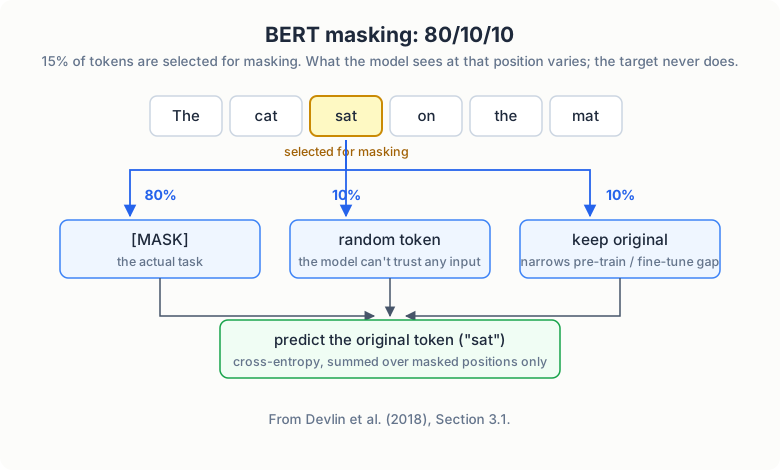
| Probability | Replacement | Why |
|---|---|---|
| 80% | [MASK] | The actual task |
| 10% | Random token | Force the model to not trust any token |
| 10% | Keep original | There is a mismatch between pre-training and fine-tuning; this reduces it |
The model predicts the original tokens at masked positions: cross-entropy over masked positions only.
Next Sentence Prediction (NSP)
50% of the time, sentence B genuinely follows A; 50% it is a random sentence. The model classifies which. (Later work suggested NSP is not necessary; RoBERTa dropped it, but we keep it for completeness.)
The code
As in the earlier chapters, what follows is the repository’s code
(model.py
and
train.py)
with the commentary docstrings trimmed. Excerpts are condensed and lightly
reformatted; the logic matches the repository.
Bidirectional attention: the one-line difference
class BidirectionalSelfAttention(nn.Module):
    # PAPER: "BERT: Pre-training of Deep Bidirectional Transformers",
    #        Devlin et al. (2018)

    def __init__(self, config):
        super().__init__()
        assert config.N_EMBD % config.N_HEAD == 0
        self.n_head = config.N_HEAD
        self.head_size = config.N_EMBD // config.N_HEAD
        self.c_attn = nn.Linear(config.N_EMBD, 3 * config.N_EMBD, bias=False)
        self.c_proj = nn.Linear(config.N_EMBD, config.N_EMBD, bias=False)
        self.attn_dropout = nn.Dropout(config.DROPOUT)
        self.resid_dropout = nn.Dropout(config.DROPOUT)
        # NOTE: no causal mask buffer. That is the entire difference from GPT.

    def forward(self, x):
        B, T, C = x.size()
        q, k, v = self.c_attn(x).split(self.n_embd, dim=2)
        k = k.view(B, T, self.n_head, self.head_size).transpose(1, 2)
        q = q.view(B, T, self.n_head, self.head_size).transpose(1, 2)
        v = v.view(B, T, self.n_head, self.head_size).transpose(1, 2)
        att = (q @ k.transpose(-2, -1)) * (self.head_size ** -0.5)

        # GPT had, right here:
        #   att = att.masked_fill(self.mask[:T, :T] == 0, float("-inf"))
        # BERT has: nothing. Every token attends to every token.

        att = F.softmax(att, dim=-1)
        att = self.attn_dropout(att)
        y = att @ v
        y = y.transpose(1, 2).contiguous().view(B, T, C)
        y = self.resid_dropout(self.c_proj(y))
        return y
The class is Chapter 1’s CausalSelfAttention with one component deleted.
That is worth internalizing: “bidirectional” is not an added mechanism, it
is the absence of a mechanism. What the model can learn with a full
attention matrix is different enough that BERT and GPT end up good at
different things, but structurally the delta is one deleted line and no
mask buffer. (The deleted line also deletes GPT’s generation ability: with
no mask, every position sees token t+1 during training, so “predict the
next token” becomes trivial and useless.)
Three embeddings summed, and two heads
        self.embeddings = nn.ModuleDict(
            dict(
                token=nn.Embedding(config.VOCAB_SIZE, config.N_EMBD),
                position=nn.Embedding(config.BLOCK_SIZE, config.N_EMBD),
                segment=nn.Embedding(2, config.N_EMBD),   # sentence A or B
                drop=nn.Dropout(config.DROPOUT),
            )
        )
        # weight tying (Press & Wolf, 2017): decode with the embedding matrix itself
        self.mlm_head = nn.Linear(config.N_EMBD, config.VOCAB_SIZE, bias=False)
        self.mlm_head.weight = self.embeddings.token.weight
        if config.USE_NSP:
            self.nsp_head = nn.Linear(config.N_EMBD, 2)
In the forward pass, the three embedding tables are summed, exactly as the BERT paper describes its input representation:
        tok_emb = self.embeddings.token(idx)
        pos = torch.arange(0, T, dtype=torch.long, device=device)
        pos_emb = self.embeddings.position(pos)
        if segment_ids is None:
            segment_ids = torch.zeros_like(idx)
        seg_emb = self.embeddings.segment(segment_ids)
        x = self.embeddings.drop(tok_emb + pos_emb + seg_emb)

        for block in self.blocks:
            x = block(x)
        x = self.ln_f(x)

        mlm_logits = self.mlm_head(x)          # (B, T, vocab_size): every position
        nsp_logits = None
        if self.config.USE_NSP:
            cls_output = x[:, 0, :]            # the [CLS] position
            nsp_logits = self.nsp_head(cls_output)
The segment embedding is the only new table versus GPT: a two-row lookup
(0 for sentence A, 1 for sentence B) added on top of token and position
embeddings, so the model can tell the two halves of a pair apart. The MLM
head projects every position to the vocabulary and is weight-tied to the
token embedding matrix, per Press & Wolf (2017); the NSP head reads only
position 0, the [CLS] slot, and answers a two-way question.
The 80/10/10 masking, in code
def mask_tokens(token_ids, tokenizer_vocab, mask_prob=0.15, mask_token_id=4,
                pad_token_id=0, unk_token_id=1, random_prob=0.1, keep_prob=0.1):
    # PAPER: BERT (2018), Section 3.1
    vocab_size = len(tokenizer_vocab)

    labels = [-100] * len(token_ids)       # -100 = ignore_index: not a target
    masked_token_ids = token_ids.copy()

    special_tokens = {0, 1, 2, 3, 4}       # never mask [PAD]/[UNK]/[CLS]/[SEP]/[MASK]
    valid_indices = [
        i for i, token_id in enumerate(token_ids) if token_id not in special_tokens
    ]
    num_to_mask = max(1, int(len(valid_indices) * mask_prob))
    mask_indices = np.random.choice(
        valid_indices, size=min(num_to_mask, len(valid_indices)), replace=False
    )

    for idx in mask_indices:
        original_token = token_ids[idx]
        labels[idx] = original_token       # the target is ALWAYS the original token

        rand = np.random.random()
        if rand < config.MASK_PROB:                        # 80%: [MASK]
            masked_token_ids[idx] = mask_token_id
        elif rand < config.MASK_PROB + config.RANDOM_PROB: # 10%: random token
            masked_token_ids[idx] = np.random.randint(5, vocab_size)
        else:                                              # 10%: keep original
            masked_token_ids[idx] = original_token

    return masked_token_ids, labels
Read the two bookkeeping lines against the figure above. The label array
starts as all -100 (PyTorch’s ignore_index), and only the positions
selected for masking get their original token written in; the loss then
ignores everything else:
        mlm_loss = F.cross_entropy(
            mlm_logits.view(-1, mlm_logits.size(-1)),
            masked_labels.view(-1),
            ignore_index=-100,             # only masked positions contribute
        )
And why replace with [MASK] only 80% of the time rather than always?
Because fine-tuning will never show the model a [MASK] token. The random
and keep-original branches force the representation of every position to
stay informative, whether or not the input happens to carry the mask
token.
Next Sentence Prediction, in code
        idx_a = np.random.randint(0, len(sentences))
        idx_b = np.random.randint(0, len(sentences))
        sent_a, sent_b = sentences[idx_a], sentences[idx_b]

        is_next = np.random.random() < 0.5
        if is_next and idx_a + 1 < len(sentences):
            sent_b = sentences[idx_a + 1]  # the genuine continuation
            label = 1                      # IsNext
        else:
            label = 0                      # NotNext (B stays the random draw above)
The pair assembly then brackets the tokens:
        input_pair = [cls_id] + tokens_a + [sep_id] + tokens_b + [sep_id]
        seg_a = [0] * (len(tokens_a) + 2)  # [CLS] and sentence A
        seg_b = [1] * (len(tokens_b) + 1)  # sentence B and the final [SEP]
A coin flip decides the label first, and only then is sentence B chosen to
match it: half the time B is replaced by the true continuation, half the
time it stays a random sentence. The segment IDs line up with the bracket
structure, [CLS] A [SEP] B [SEP], which is what the segment-embedding
table from the previous section consumes.
Configuration
config.py documents every choice against the paper. The demonstration
model is deliberately small:
| Hyperparameter | BERT-base | This project |
|---|---|---|
| Layers | 12 | 6 |
| Hidden size | 768 | 256 |
| Heads | 12 | 8 |
| Params | 110M | ~4.8M |
| MLM probability | 15% | 15% |
Running it
uv run python phase1_foundation/project3_contextual_embeddings/download_data.py --size small
uv run python phase1_foundation/project3_contextual_embeddings/train.py
Checkpoints land in checkpoints/project3/ as bert_iter{N}_loss{L}.pt
containing model + optimizer state and the loss. On the RTX 3050, 10,000
iterations train in about 12 minutes, with MLM loss falling from 4.2 to
around 1.4.
Code tour
| File | What to read |
|---|---|
model.py | BidirectionalSelfAttention (no causal mask!), TransformerEncoderBlock, the BERT class |
train.py | mask_tokens (the 80/10/10 scheme), NSP pair construction, the training loop |
config.py | All hyperparameters with paper quotes |
Exercises
- Set
MLM_PROBto 0.5: how does training stability change? - Disable the random-token branch (make it 90/10/0) and compare MLM loss.
- (Concept) Why can’t this model generate text? Trace the forward pass.
What’s next
A pre-trained encoder produces token embeddings. Chapter 4 shapes them into sentence embeddings with contrastive learning, where the data augmentation is dropout itself.
SimCSE: Sentence Embeddings
Project source:
phase1_foundation/project3b_simcse/Papers: “SimCSE: Simple Contrastive Learning of Sentence Embeddings” (Gao, Yao & Chen, EMNLP 2021) · “Understanding Contrastive Representation Learning through Alignment and Uniformity on the Hypersphere” (Wang & Isola, 2020) · STS-B (Cer et al., 2017)
The problem
Chapter 3’s encoder produces contextual token embeddings. Downstream tasks (semantic search, clustering, duplicate detection) need a single vector per sentence where similar sentences end up close together. Averaging the encoder’s outputs doesn’t give you that geometry.
SimCSE fixes it with an almost absurdly simple recipe:
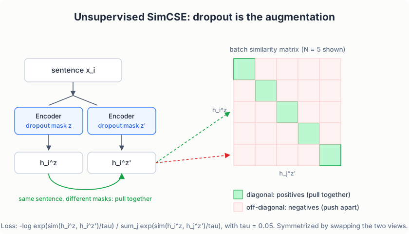
Feed the same sentence into the encoder twice. Because dropout masks are sampled independently, you get two slightly different embeddings. Train the encoder to pull those two together and push every other sentence in the batch away.
No paraphrase data, no translation pairs. Dropout is the data augmentation. The paper puts it plainly:
“dropout acts as minimal data augmentation, and removing it leads to a representation collapse.”
The objective
For a mini-batch of N sentences (equation 4 of the paper):
                  exp(sim(h_i^z, h_i^z')/τ)
l_i = -log -------------------------------------------
           Σ_j exp(sim(h_i^z, h_j^z')/τ)
| Symbol | Meaning |
|---|---|
h_i^z | Embedding of sentence x_i under dropout mask z |
h_i^z' | The same sentence under an independent mask z' |
sim(·,·) | Cosine similarity |
τ | Temperature, 0.05 for unsupervised SimCSE |
This is an N-way classification over the batch: each row of the similarity matrix must find its own positive on the diagonal. The loss is symmetrized by swapping the two views.
Why it works: alignment and uniformity
Wang & Isola (2020) characterize good contrastive spaces with two metrics
(both implemented in model.py):
- Alignment: similar sentences map to nearby points (positives are close)
- Uniformity: embeddings spread evenly over the hypersphere
The paper’s diagnostic: models with no dropout, or with a fixed dropout mask shared by both copies, trivially make the two views identical. Their alignment collapses to zero but their representations clump, so uniformity is destroyed and STS-B degrades dramatically. Independent dropout masks keep alignment steady while still improving uniformity. Starting from a pre-trained checkpoint matters too: “it provides good initial alignment.”
The “MLP trick”
During training, a one-layer MLP with tanh sits on top of the [CLS]
embedding, and the contrastive pressure flows through it. At evaluation
the head is discarded and the raw [CLS] embedding is used, which is worth
1–2 Spearman points. The intuition: let the loss shape the space through a
disposable projection, leaving the underlying embedding closer to its
pre-trained manifold.
The code
This is the repository’s code
(model.py,
train.py,
evaluate.py)
with the commentary docstrings trimmed. Excerpts are condensed and lightly
reformatted; the logic matches the repository.
Equation 4, in code
def simcse_loss(z1, z2, temperature):
    # PAPER: SimCSE, Gao et al. (2021), equation 4
    z1 = F.normalize(z1, p=2, dim=-1)      # L2-normalize: dot product == cosine
    z2 = F.normalize(z2, p=2, dim=-1)

    sim_12 = z1 @ z2.t() / temperature     # (N, N) scaled cosine similarities
    sim_21 = z2 @ z1.t() / temperature     # the same matrix, views swapped

    labels = torch.arange(z1.size(0), device=z1.device)  # positive of row i is column i

    loss_12 = F.cross_entropy(sim_12, labels)
    loss_21 = F.cross_entropy(sim_21, labels)
    return (loss_12 + loss_21) / 2
Map each line onto the formula from the objective section. Normalizing
both views to unit length turns the dot product into cosine similarity.
z1 @ z2.t() builds the whole batch similarity matrix at once; dividing
by τ = 0.05 stretches it twenty-fold, which is what makes off-diagonal
negatives hard (their similarities differ by fractions, but after
scaling those fractions are the entire game). The labels are the identity:
row i must pick out column i, its own re-encoding. And because
F.cross_entropy computes -log softmax over each row, the denominator
of equation 4, the sum over all j, is exactly what softmax normalizes
against. The symmetrization at the end trains both directions.
The two forward passes
            # Two forward passes = two independent dropout masks (the
            # entire "augmentation" of unsupervised SimCSE)
            z1 = encoder.encode(idx, attention_mask, project=config.USE_MLP_HEAD)
            z2 = encoder.encode(idx, attention_mask, project=config.USE_MLP_HEAD)

            loss = simcse_loss(z1, z2, config.TEMPERATURE)
Earlier in the same function there is encoder.train() # dropout ON - it IS the augmentation. That comment is the whole method: same batch, same
tokens, no other transformation, two calls. Every stochastic layer inside
the encoder (attention dropout, residual dropout, embedding dropout)
resamples its mask independently on each call, and the gap between the two
embeddings is the positive pair the loss pulls together. If the encoder is
put in eval mode, both calls return the identical tensor, the loss is
log(N), and nothing is learned.
The MLP head and pooling
class MLPHead(nn.Module):
    # PAPER: Gao et al. (2021): "an MLP layer (with one tanh activation) on
    # top of the [CLS] representation ... used only for training but not
    # for evaluation"
    def __init__(self, n_embd):
        super().__init__()
        self.dense = nn.Linear(n_embd, n_embd)
        self.activation = nn.Tanh()

    def forward(self, cls_hidden):
        return self.activation(self.dense(cls_hidden))
        if self.pooler == "cls":
            emb = hidden[:, 0, :]              # the [CLS] hidden state
        elif self.pooler == "mean":
            mask = attention_mask.unsqueeze(-1).float()
            emb = (hidden * mask).sum(dim=1) / mask.sum(dim=1).clamp(min=1.0)
        else:
            raise ValueError(f"Unknown pooler: {self.pooler}")

        if project:                            # training only: the MLP trick
            emb = self.mlp_head(emb)
        return emb
The project flag is where the train/eval asymmetry lives: training
passes route the contrastive pressure through the disposable projection,
evaluation calls encode(..., project=False) and uses the raw [CLS]
embedding. Mean pooling exists as the comparison baseline; it excludes
[PAD] positions via the attention mask so padding cannot dilute the
average.
Alignment and uniformity
def alignment_and_uniformity(z1, z2, temperature=0.05):
    # Wang & Isola (2020); SimCSE Section 3 uses these to explain WHY dropout works
    z1 = F.normalize(z1, p=2, dim=-1)
    z2 = F.normalize(z2, p=2, dim=-1)

    alignment = (z1 - z2).norm(p=2, dim=-1).pow(2).mean().item()

    all_z = torch.cat([z1, z2], dim=0)
    sq_pdist = torch.pdist(all_z, p=2).pow(2)
    uniformity = (-sq_pdist.mul(-2.0 * temperature).exp().mean().log()).item()
    return alignment, uniformity
Both numbers read “lower is better”. Alignment is the mean squared distance between positive pairs; uniformity is a soft measure of how evenly all embeddings spread over the sphere. They are diagnostics, not losses: the collapse the paper warns about shows up as alignment crashing toward zero while uniformity explodes, which is precisely what you observe if you run the exercise with dropout disabled.
The evaluation protocol
@torch.no_grad()
def evaluate_stsb(encoder, split="validation", device=None):
    s1, s2, gold = load_sts_b(split)

    emb1 = encode_sentences(encoder, s1, device=device)   # eval mode: dropout OFF
    emb2 = encode_sentences(encoder, s2, device=device)   # no MLP head either

    e1 = F.normalize(torch.from_numpy(emb1), p=2, dim=-1)
    e2 = F.normalize(torch.from_numpy(emb2), p=2, dim=-1)
    cosine = (e1 * e2).sum(dim=-1).numpy()

    spearman = spearmanr(cosine, gold).statistic
    return float(spearman) * 100
The three contract points from the paper are all visible here. Dropout is
off (encode_sentences calls encoder.eval()), so scores are
reproducible. The MLP head is bypassed. And the reported number is
Spearman, not Pearson: STS-B quality is judged by whether the model’s
ranking of sentence pairs agrees with the human ranking, so what matters
is the correlation between ranks, not raw values.
Evaluation: STS-B
The Semantic Textual Similarity Benchmark (Cer et al., 2017) provides 1,500 dev sentence pairs scored 0–5 by humans. Encode both sentences of every pair (dropout OFF, deterministic), compute cosine similarity, and report the Spearman rank correlation with the human scores. The paper’s BERT-base result: 82.5 dev Spearman.
Note: the GLUE test split’s labels are hidden (leaderboard only), so the dev split is the reportable number.
Results
Trained on 100k Wikipedia sentences, batch 64, τ = 0.05, lr 5e-5, max sequence length 32, on an RTX 3050:
| Model | STS-B dev Spearman |
|---|---|
Project 3 MLM encoder, raw [CLS] (baseline) | 16.6 |
| SimCSE, 1 epoch | 27.0 |
| SimCSE, 3 epochs (final) | 34.7 |
| SimCSE, 5 epochs (overfits) | 33.5 |
That is +18.1 Spearman over the baseline. The paper’s number is higher because their model has 110M parameters and 10⁶ sentences; the pipeline here is theirs, unchanged. Each epoch takes about 26 seconds on the GPU, so hyperparameter experiments are cheap.
Running it
# Sentence corpus + STS-B
uv run python phase1_foundation/project3b_simcse/download_data.py

# Sanity-test the mechanics before training (runs anywhere, seconds)
uv run python phase1_foundation/project3b_simcse/test_model.py

# Train, then evaluate
uv run python phase1_foundation/project3b_simcse/train.py
uv run python phase1_foundation/project3b_simcse/evaluate.py
The sanity tests verify the machinery itself: two forward passes with dropout ON produce different embeddings (if not, the positive pair is degenerate); aligned positives yield lower loss than misaligned ones; gradients reach both the encoder and the MLP head.
Code tour
| File | What to read |
|---|---|
model.py | SimCSEEncoder (wraps Project 3’s BERT), MLPHead, simcse_loss, alignment_and_uniformity |
data.py | Sentence loading, [CLS] s [SEP] [PAD] batching |
train.py | Two-view training loop, warmup + linear decay |
evaluate.py | STS-B protocol |
test_model.py | The sanity suite |
Exercises
- Turn dropout off (
p=0) and retrain. Watch the collapse the paper predicts (Section 3, Table 3). - Swap
[CLS]pooling for mean pooling. Which wins at this scale? - Train on the full extracted corpus (raise
MAX_SENTENCES): does more data close the gap faster than more epochs?
What’s next
Phase 2 applies the same from-scratch discipline to fine-tuning: SFT, LoRA, and DPO. Phase 3 then makes inference fast: mixed precision, KV-cache, and Flash Attention.
Pre-Training a 125M GPT
Project source:
phase1_foundation/project4_pretrain/Papers: “Language Models are Unsupervised Multitask Learners” (Radford et al., 2019, GPT-2) · “Language Models are Few-Shot Learners” (Brown et al., 2020, GPT-3) · “Training Compute-Optimal Large Language Models” (Hoffmann et al., 2022, Chinchilla) · “FlashAttention” (Dao et al., 2022) · WikiText (Merity et al., 2016)
From 10M to 125M
Everything Phase 2 does to a language model (SFT, LoRA, DPO) assumes there is a base model worth fine-tuning. The chapter 1 GPT, at 10M parameters trained on 1M characters of Shakespeare, is a demo of the architecture. A base model needs to have seen two or three orders of magnitude more text. This chapter builds that model: the same decoder-only stack from chapter 1, scaled up to GPT-2-small class and pre-trained on WikiText-103.
The target size comes from GPT-2. Its smallest released model has 124M parameters (12 layers, 768 hidden, 12 heads, 50,257-token BPE vocabulary). Chinchilla (Hoffmann et al., 2022) says a compute-optimal 124M model wants roughly 20 tokens per parameter, about 2.5B tokens of training. Our budget is one RTX 3050 for a few hours, which buys ~131M tokens, about one pass over WikiText-103. That is 5% of the compute-optimal dose, and the loss numbers at the end reflect it. The point of the chapter is the machinery; once it exists, extra tokens are just measured throughput times more hours.
Counting the parameters exposes a vocabulary problem. GPT-2’s 50,257-token embedding table accounts for 38.6M of its 124M parameters, nearly a third. Our from-scratch BPE from chapter 2 targets a 16,384-token vocabulary, which makes the embedding table only 12.6M parameters. Keeping GPT-2’s 12 layers would land the model at 98M. Raising it to 16 layers lands at 126,273,024, GPT-2-small class with our own tokenizer:
| Component | Count |
|---|---|
Token embedding wte (16,384 × 768, tied with output head) | 12,582,912 |
Position embedding wpe (512 × 768) | 393,216 |
| 16 transformer blocks (7,080,960 each) | 113,295,360 |
| Final LayerNorm | 1,536 |
| Total | 126,273,024 |
Depth for vocabulary is a reasonable trade at this scale: GPT-2’s own model
family scales depth before width, and attention/MLP widths stay identical
to GPT-2 small. The one behavioral difference is a smaller vocabulary, and
test_model.py asserts the total parameter count so the number above stays
honest.
Training the tokenizer at WikiText-103 scale
Chapter 2’s tokenizer needs retraining here, for two reasons. A 5,000-token vocabulary fragments WikiText-103 into long token sequences, which slows training directly (more tokens per document). And the corpus is 45× bigger than WikiText-2, which breaks the training loop itself.
The chapter 2 trainer recomputes pair counts over every distinct word at
every merge. On WikiText-2 that cost ~12 minutes for 3,983 merges, using
the distinct-words-with-multiplicities trick. Scale the corpus 45× and the
merge count 4× and the same loop needs the better part of a day. The
optimizer in tokenizer.py keeps the same objective, repeatedly merge the
most frequent adjacent pair, but updates the counts incrementally. Three
data structures do it:
pair_counts: how often each adjacent pair occurs, weighted by word frequencypair_to_words: which word indices contain each pair- a max-heap of
(-count, pair)entries for finding the most frequent pair without rescanning
At each merge, only words that actually contain the winning pair get touched. Their old pair contributions are subtracted, the merge is applied to their symbols, and the new contributions are added back. Everything else in the corpus is irrelevant to this merge, and the index makes that literally true instead of approximately.
The heap has one subtlety worth dwelling on. Counts change constantly, and a heap cannot be updated in place, so the trainer pushes a fresh entry on every count change and skips stale entries when they pop:
# pop the most frequent pair, skipping stale heap entries
best_pair = None
while heap:
    neg_count, pair = heapq.heappop(heap)
    # fresh only if it still matches the live count
    if pair_counts.get(pair) == -neg_count:
        best_pair = pair
        best_freq = -neg_count
        break
An entry is trusted only when its count matches the live pair_counts.
That check is also a bug trap: the first version of this loop pushed new
entries only on increments, so a pair whose count had only decreased had
no fresh entry left and became invisible to the trainer even while still
frequent. The naive-vs-incremental test caught it (more on that test
below), and the fix was to push after every change, decrements included.
Ties break differently from chapter 2. There, max() over a dict broke
ties by insertion order, which is deterministic but awkward to reproduce in
a test. Here the heap orders by (-count, pair), so among equal counts the
lexicographically smallest pair wins. Different tie-breaks produce
different, equally valid BPE vocabularies; the deterministic one is
testable.
The naive trainer still earns its keep in tests: at test scale it is
cheap, so test_model.py implements it as a reference (full rescan every
merge, same lexicographic tie-break) and asserts the merge lists are
identical:
✓ Incremental trainer matches naive rescan (116 identical merges)
Encoding needed its own fix. Chapter 2’s encode applies every learned
merge to the whole text, O(merges × length) per call. Fine for a sentence,
hopeless for 540 MB. The standard trick (GPT-2’s encoder.py, tiktoken)
replaces it: find the adjacent pair with the lowest merge rank, merge all
its occurrences, repeat. This is provably the same result as applying
merges in learned order, because any pair created by merge k can only
participate in merges with rank greater than k. Per-word memoization on
top means a 540 MB corpus costs one pass plus a few hundred thousand
dictionary lookups.
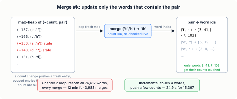
The measured gap, on WikiText-2 so both runs see the same corpus: 3,983 merges in ~12 minutes for the chapter 2 loop versus 15,367 merges in 24.9 seconds for the incremental one, more than 100× as many merges per minute. Training the full 16,384-token tokenizer on a 100 MB sample of WikiText-103 then takes about two minutes instead of a day.
The data pipeline
WikiText-103 arrives as three text files (wiki.train.raw, 540 MB among
them) organized in articles, with headings on lines that start with
=. prepare_data.py splits at those heading lines, wraps every
article in <BOS> … <EOS>, and encodes it with the tokenizer.
The boundary tokens matter because of a convention inherited from chapter
2: the tokenizer’s word normalization collapses all whitespace, so newlines
do not survive encoding. Without explicit <BOS>/<EOS> the token stream
would be one endless document and the model would never see article
boundaries. The special token IDs (0 = <PAD>, 1 = <UNK>, 2 = <BOS>,
3 = <EOS>) are the same ones chapters 3 and 4 build on.
Each split becomes one flat array of uint16:
    for doc in tqdm(docs, desc=f"encoding {split_name}", unit="doc"):
        ids.append(BOS)
        ids.extend(tokenizer.encode(doc))
        ids.append(EOS)

    array = np.asarray(ids, dtype=np.uint16)
uint16 works because 16,384 < 65,536 (config asserts this), and it halves the file size versus uint32. GPT-2’s 50,257-token vocabulary would not fit in 16 bits, one more reason the vocabulary choice is not arbitrary. Training later memory-maps these files and samples random 512-token windows: no padding, no per-step tokenization, and the corpus never sits in RAM.
What changes in the model
The block structure is unchanged from chapter 1: pre-LN, causal self-attention, 4× GELU MLP, residuals. Three things change, each because of the scale.
Fused attention. Chapter 1 computes attention the way the paper writes
it: scores QKᵀ/√d_k, mask, softmax, multiply by V. At this size that
materialized score matrix is the bottleneck. One layer’s scores for one
batch are 8 × 12 × 512 × 512 floats, about 100 MB, and backward needs them
per layer. F.scaled_dot_product_attention (PyTorch’s implementation of
the FlashAttention strategy, Dao et al. 2022) computes the same function
without ever storing the matrix:
        # fused causal attention: softmax(q k^T / sqrt(d_k)) v with the
        # upper triangle masked out. dropout_p regularizes attention
        # weights during training only.
        y = F.scaled_dot_product_attention(
            q, k, v,
            dropout_p=self.attn_dropout if self.training else 0.0,
            is_causal=True,
        )
Same math as the chapter 1 version (chapter 1’s is kept as the reference implementation), tiles instead of a materialized matrix.
Residual-scaled initialization. GPT-2’s released code initializes weights as Normal(0, 0.02), except the two projections in each block whose output feeds the residual stream, which get 0.02/√(2·N_LAYER). The reason: the residual stream accumulates one contribution per layer, so its variance at initialization grows like depth. Scaling each contribution by 1/√depth keeps the stream’s variance flat across 16 layers, cheap insurance for a stack this deep.
    def _init_weights(self, module):
        if isinstance(module, nn.Linear):
            std = 0.02
            if getattr(module, "_is_residual", False):
                std /= (2 * self.config.N_LAYER) ** 0.5
Weight tying. The output projection lm_head shares its weight matrix
with wte (Press & Wolf, 2017; GPT-2 does the same). It saves 12.6M
parameters, the entire vocabulary-sized matrix, and for small-vocabulary
models it usually helps perplexity too.
One more visible choice: no bias terms on the attention and MLP linears. GPT-2 kept them; GPT-3 and most runs since dropped them with no measurable loss, and each removed bias is one less thing to allocate and update.
The training loop
The chapter 1 loop is batch → forward → backward → step, and that shape
survives. What changes is the arithmetic around it.
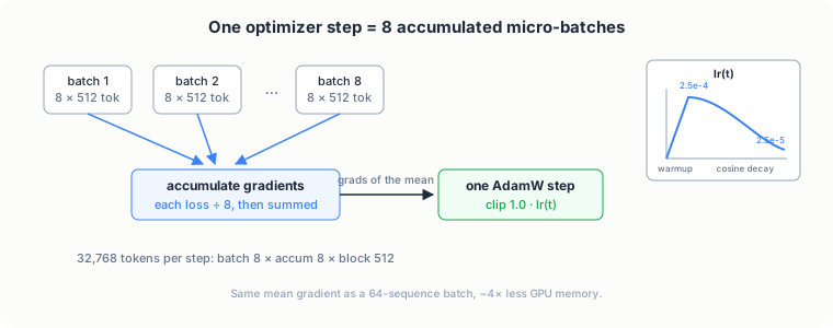
Gradient accumulation. GPT-3’s smallest model trains on batches of about 0.5M tokens. An 8 GB card fits perhaps 4,000. Gradient accumulation splits the logical batch into micro-batches: forward and backward through 8 sequences of 512 tokens at a time, 8 times, summing scaled gradients, then stepping once. Dividing each loss by the number of micro-batches makes the accumulated gradient the gradient of the mean loss, identical to a true 64-sequence batch:
        optimizer.zero_grad(set_to_none=True)
        for _ in range(config.GRAD_ACCUM_STEPS):
            x, y = get_batch(train_data, config.BATCH_SIZE, config.BLOCK_SIZE,
                             config.DEVICE)
            with autocast_ctx():
                _, loss = model(x, y)
            # scale so the accumulated gradient equals the mean over all
            # micro-batches, not the sum
            (loss / config.GRAD_ACCUM_STEPS).backward()
        torch.nn.utils.clip_grad_norm_(model.parameters(), config.GRAD_CLIP)
        optimizer.step()
That is 32,768 tokens per optimizer step at batch 8, which fits memory with room to spare.
bf16 mixed precision. Forward and backward run in bfloat16, master weights and AdamW moments stay in fp32. bf16 has the same exponent range as fp32, so activations do not overflow the way they can in fp16, and there is no loss scaler to tune. The RTX 3050 (Ampere) runs bf16 natively.
Learning rate schedule. GPT-3’s recipe: linear warmup, then cosine decay to 10% of peak. Warmup exists because Adam’s second-moment estimates are garbage during the first steps; taking 2.5e-4-sized steps on garbage variance estimates is how training runs die in iteration 50.
def get_lr(it: int) -> float:
    if it < config.WARMUP_ITERS:
        return config.LEARNING_RATE * (it + 1) / config.WARMUP_ITERS
    if it >= config.MAX_ITERS:
        return config.MIN_LEARNING_RATE
    progress = (it - config.WARMUP_ITERS) / (config.MAX_ITERS - config.WARMUP_ITERS)
    cos = 0.5 * (1 + math.cos(math.pi * progress))
    return config.MIN_LEARNING_RATE + cos * (config.LEARNING_RATE - config.MIN_LEARNING_RATE)
Weight decay (0.1) applies to weight matrices only, not to LayerNorm gains, per GPT-3 Appendix B. Gradient clipping at global norm 1.0 keeps one bad batch from poisoning the optimizer’s moment estimates.
Checkpointing keeps the repository-wide five-key format (iter,
model, optimizer, train/val loss) in checkpoint_latest.pt every 100
steps, with checkpoint_best.pt tracking the best validation loss, and
--resume continues from the latest snapshot. Loads use
torch.load(..., weights_only=True), which refuses anything but tensors
and primitives.
Results
The run: 4,000 optimizer steps at 32,768 tokens each, ~131M tokens, one pass over the 123.5M-token train split. bf16, batch 8 × accumulation 8 × block 512. Wall time was 2 hours 36 minutes on the RTX 3050 at a steady 14,100 tokens/second (the smoke estimate from a 3-step run was 5,700; the first few hundred steps are slower while kernels warm up), using 5.8 GB of the 8 GB of GPU memory.
| Iter | Val loss | Val perplexity |
|---|---|---|
| 0 | 9.83 | ~18,500 |
| 500 | 5.12 | 167 |
| 1,000 | 4.39 | 80.4 |
| 2,000 | 3.73 | 41.8 |
| 3,000 | 3.51 | 33.5 |
| 3,800 (best checkpoint) | 3.39 | 29.5 |
| 3,999 (final) | 3.41 | 30.2 |
Validation loss improved at every evaluation until the last few hundred steps, where the flat learning rate and the single-pass data budget show up as small oscillations. The best checkpoint (iter 3,800, val loss 3.385) is the one to fine-tune from.
Text sampled from <BOS> at the end of the run:
= = History = = This first recorded reference to the song was recorded by Paul McCartney at the Abbey Road Abbey in London on 19 April 1967 . The song was recorded at the Abbey Road Studios in London in April 1968 . … “ Cry Me a New Moon “ was the third single from the album .
The register is right: article headings, dated statements, the flat Wikipedia voice. The facts are confabulated, as they should be for a model that has seen the equivalent of one pass over its corpus. This is the checkpoint Phase 2 starts from.
One caution when comparing numbers. GPT-2’s paper reports 37.5 perplexity on WikiText-103 for the 124M model. Our 30.2 is not better than that: GPT-2’s number is zero-shot, evaluating on WikiText-103 a model trained on a different corpus (WebText) with a different tokenizer, while ours is in-domain, trained on WikiText-103 with a tokenizer trained on the same corpus. The two setups answer different questions, and the honest summary of ours is: 131M tokens took a 126M parameter model from random (perplexity ~18,500) to 30, on one consumer GPU in an afternoon. The Chinchilla-optimal run would need ~2.5B tokens, about 19× more, which at 14,100 tokens/second is roughly 50 hours of the same GPU.
Running it
# 1. corpus (~190 MB download)
uv run python phase1_foundation/project4_pretrain/download_data.py --size full
#    (--size small fetches WikiText-2-raw, ~5 MB, for smoke tests)

# 2. tokenizer (16,384 vocab from a seeded 100 MB sample)
uv run python phase1_foundation/project4_pretrain/train_tokenizer.py

# 3. encode splits to uint16 token files
uv run python phase1_foundation/project4_pretrain/prepare_data.py

# 4. sanity-check everything
uv run python phase1_foundation/project4_pretrain/test_model.py

# 5. pre-train (default 4,000 steps; interrupt-safe)
uv run python phase1_foundation/project4_pretrain/train.py
uv run python phase1_foundation/project4_pretrain/train.py --resume   # continue

# 6. sample
uv run python phase1_foundation/project4_pretrain/generate.py --prompt "The theory"
The sanity tests verify the parts that are hard to see from loss curves: the incremental trainer produces exactly the naive algorithm’s merge list, the rank-based encoder equals ordered-merge encoding, future tokens cannot change past logits, and a checkpoint round-trips to identical logits.
Code tour
| File | What to read |
|---|---|
config.py | Every hyperparameter with its paper reference; the 12→16 layer note |
tokenizer.py | Incremental BPE trainer (heap + lazy deletion), rank-based encode |
train_tokenizer.py | Seeded corpus sampling |
prepare_data.py | Document boundaries, uint16 bins |
model.py | SDPA attention, GPT-2 init, weight tying |
train.py | bf16 + accumulation loop, warmup/cosine, checkpointing |
generate.py | Sampling CLI |
test_model.py | The sanity suite, incl. incremental-vs-naive equivalence |
Exercises
- Set
BLOCK_SIZE = 1024(GPT-2’s value) and re-measure throughput. Is the halving from the context length or the attention matrix? - Train a 32,768-token tokenizer. How much does compression (characters per token) improve, and what does it cost in embedding parameters if you keep 16 layers?
- Overfit one batch on purpose (batch 2, one repeated window, a few hundred steps). Confirm the loss approaches zero; if it doesn’t, the pipeline has a bug no schedule can fix.
- The model is 5% of Chinchilla-optimal on tokens. Estimate (from the measured tokens/s) how many days 2.5B tokens takes, then estimate what a 4-layer 30M version would need. Which direction would you scale first?
What’s next
Phase 2 starts with this checkpoint: supervised fine-tuning on instruction data (Project 5), then LoRA (Project 6) and DPO (Project 7) all attach to the base model trained here.
Supervised Fine-Tuning
Project source:
phase2_finetuning/project5_sft/Papers: “Training Language Models to Follow Instructions with Human Feedback” (Ouyang et al., 2022, InstructGPT) · “Stanford Alpaca: An Instruction-following Llama Model” (Taori et al., 2023) · “Self-Instruct: Aligning Language Models with Self-Generated Instructions” (Wang et al., 2023) · “Finetuned Language Models Are Zero-Shot Learners” (Wei et al., 2022, FLAN) · “LIMA: Less Is More for Alignment” (Zhou et al., 2023)
The base model can only continue
Ask the chapter 5 model “What is the capital of France?” and it does the only thing it was ever taught: it continues the text. Somewhere in its training distribution a passage listing cities follows, and that is what you get, in Wikipedia’s dated voice, with confabulated facts. The model is not broken. It has simply never seen a question that expected an answer.
Fixing this is the first stage of the alignment recipe from InstructGPT (Ouyang et al., 2022): collect (instruction, response) pairs, fine-tune the base model on them (SFT), then train a reward model and optimize against it (RLHF, projects 7 and beyond in spirit). This chapter builds stage one. LoRA and DPO in the coming chapters attach to the checkpoint this one produces.
The appealing surprise is how little changes. The architecture moves not
at all: model.py in project 5 is the same code as project 4, and the
parameter count stays 126,273,024. What changes is the data, the loss
mask, and the learning rate. SFT is a nudge, a few percent as many
optimizer steps as pre-training, applied to weights that already sit in a
good basin. The nudge is what makes a text-continuer into something that
answers.
Instruction data: 52,000 Alpaca triples
The dataset is Stanford Alpaca (Taori et al., 2023): 52,002 triples of
instruction, optional input, and output, generated with
Self-Instruct (Wang et al., 2023) from 175 seed tasks written by hand.
The instruction asks for something, the input supplies optional context,
the output is the desired response:
instruction: What is the capital of France?
input:       (empty)
output:      The capital of France is Paris.
Twenty-eight entries have empty outputs and carry no supervised signal,
so 51,974 survive. A seeded shuffle holds out the last 1,000 for
validation: 50,973 train, 1,000 val. Averages on the train split: 65.8
prompt tokens and 70.3 response tokens per example, 0.003% <UNK>. The
whole set encodes in about 33 seconds at roughly 1,600 examples per
second, because the chapter 4 tokenizer memoizes per-word encodings.
Each triple renders into one prompt with Alpaca’s plain-text markers:
Below is an instruction that describes a task. Write a response that
appropriately completes the request.

### Instruction:
What is the capital of France?

### Response:
No new special tokens. Adding <|assistant|>-style markers would force
an embedding-table resize, which touches the base model’s weights before
training even starts. The base tokenizer read 100 MB of English prose in
chapter 5 and knows every character in ### Instruction: already, so plain-text markers cost nothing and “SFT
attaches to the base model unchanged” stays literally true. The
termination signal does use a reserved token: a <EOS> (id 3) after the
response, which the sampler learns to listen for.
One honest limitation, inherited from the tokenizer: it normalizes
whitespace, because WikiText is a word stream and
chapter 5’s prepare_data.py added document
boundaries explicitly. Every formatted example therefore encodes as one
long line. The ### markers carry the structure; the model never learns
newline placement. Code-heavy Alpaca outputs decode as run-on text. A
tokenizer with byte-level fallback and preserved newlines is the fix, and
it is deliberately left to a later project.
The response mask
Pre-training computes the loss at every position: each token predicts the
next one, and the model learns the statistics of the whole stream,
prompts included. Keep that objective for instruction data and the model
learns something you did not ask for: that a ### Response: block is
usually followed by another ### Instruction: block. It memorizes the
format of the conversation and keeps writing new instructions after
answering, because that is what the loss rewarded.
SFT computes the loss on the response only. The mechanism already exists
in the chapter 1 loss: F.cross_entropy takes an
ignore_index, and positions whose target is -1 contribute nothing.
So each example becomes two aligned arrays:
tokens:<BOS>, the prompt, the response,<EOS>, then<PAD>up to length 512labels:-1everywhere except the response and the<EOS>, which carry the token to teach
The training batch applies the same shift as every chapter: input
position t holds token t, target position t holds the label for
token t + 1. Two consequences worth pausing on. The last prompt token
must predict the first response token, which is exactly the skill
“answer the question”. And the last response token must predict <EOS>,
which is exactly the skill “know when to stop”.
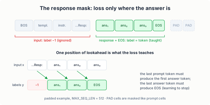
<EOS> teach answering and stopping.A real example, encoded with the chapter 5 tokenizer: the prompt above
(49 prompt tokens), the response “The capital of France is Paris.” (8
response tokens), 59 real positions including <BOS> and <EOS>. The
taught span is positions 50 through 58, nine positions, and decoding
exactly those label positions gives back “The capital of France is
Paris.”. Everything before position 50 is input.
Both papers behind this project agree the loss matters and disagree on
where it applies. InstructGPT computes the SFT loss only on assistant
tokens; Alpaca’s released code trains on the full sequence, prompt
included, and works anyway. train.py --loss_on {response,full} makes
the comparison one flag (default: response); exercise 1 runs it.
The trailing-space junction
Masking needs to know where the response starts, and our tokenizer makes
that subtle. Its tokens include trailing spaces (“the “ is one token),
and a word encodes differently depending on whether another word follows
it: Response: at the end of a string and Response: mid-stream are
different token sequences. Splicing token lists by position, encoding
the prompt and hoping it is a prefix of the full encoding, breaks at
exactly this junction. Measured on the example above:
encode(prompt) is a prefix of encode(prompt + " " + output):  False
encode_words(prompt, final=False) + encode_words(response, final=True)
        == encode(prompt + " " + output):                     True
So template.encode_labeled() splits both halves into words and encodes
each with the trailing-space convention applied explicitly: every prompt
word keeps its trailing space (the response always follows it), only the
final response word drops it. Because encoding is per-word and
context-free, the concatenation is exactly the one-shot encoding of the
whole text, and test_model.py asserts that identity so the guarantee
cannot rot silently.
Attaching to the base checkpoint
Training starts from checkpoints/project4/model_final.pt (iter 3,999,
val loss 3.408), loaded with the same weights_only=True discipline as
every checkpoint in this repository:
ckpt = torch.load(path, map_location="cpu", weights_only=True)
arch = ckpt.get("config")
...
model = GPT(GPTConfig(
    VOCAB_SIZE=arch["VOCAB_SIZE"],
    N_EMBD=arch["N_EMBD"],
    N_HEAD=arch["N_HEAD"],
    N_LAYER=arch["N_LAYER"],
    BLOCK_SIZE=arch["BLOCK_SIZE"],
    DROPOUT=arch.get("DROPOUT", 0.0),
))
model.load_state_dict(ckpt["model_state_dict"])
No key translation is needed anywhere in that load, which is the point
of keeping model.py code-identical to project 4’s.
The optimizer starts fresh even though the weights do not. AdamW’s second-moment estimates describe the pre-training gradient landscape and mean nothing about the fine-tuning one, so the first steps get a short warmup (100 iterations) for the same reason pre-training did.
The learning rate drops from 2.5e-4 to 2e-5, Alpaca’s setting and a 12x
reduction. The base weights encode a distribution that took 131M tokens
to learn; a few large steps damage it faster than the new behavior can
replace it, which is the catastrophic-forgetting trap. Three epochs over
51k examples is short enough that overfitting, not underfitting, is the
failure mode to watch, so the loop tracks a val estimate every 100 steps
and keeps checkpoint_best.pt by val loss. The rest of the loop is the
chapter 5 skeleton unchanged: bf16 autocast, gradient accumulation
(8 x 8 = 64 examples per step), grad clipping at 1.0, cosine decay to
10% of peak, five-key checkpoints. Dropout stays at 0.0 for the same
reason as pre-training: the schedule is short and the data is not tiny.
The code
Encoding one example
template.py owns the template and the mask arithmetic. Everything
downstream (prepare, train, generate, tests) goes through it:
prompt_ids = tokenizer.encode_words(prompt_text.split(), final=False)
response_ids = tokenizer.encode_words(output.split(), final=True)

response_start = len(prompt_ids) + 1
if response_start + 2 > max_seq_len:  # +2: one response token + <EOS>
    raise ValueError(
        f"prompt needs {response_start} of {max_seq_len} positions; "
        f"no room for a response"
    )

tokens = [bos] + prompt_ids + response_ids
if len(tokens) >= max_seq_len:
    # truncate the RESPONSE to fit; the prompt stays intact and <EOS>
    # closes whatever response remains
    tokens = tokens[:max_seq_len - 1] + [eos]
else:
    tokens.append(eos)
tokens = tokens + [pad] * (max_seq_len - len(tokens))

labels = [-1] * len(tokens)
for i in range(response_start, len(tokens)):
    if tokens[i] != pad:
        labels[i] = tokens[i]
return tokens, labels
Truncation cuts the response, never the prompt. Losing the end of an answer is acceptable; losing the question is not.
Building the batch
The shift happens at batch time in train.py, and the loss mode is a
one-line switch:
idx = np.asarray(indices, dtype=np.int64)
x = rows[idx][:, :-1].astype(np.int64)
y = (labels[idx][:, 1:] if loss_mode == "response" else rows[idx][:, 1:]).astype(np.int64)
return torch.from_numpy(x).pin_memory(), torch.from_numpy(y).pin_memory()
loss_mode == "full" simply drops the mask: targets become the raw
tokens, Alpaca’s own choice. One subtlety the tests pin down: the numpy
.astype returns a fresh C-contiguous copy, which model.forward’s
fused cross-entropy requires (it calls .view(-1) on the targets, and
.view refuses non-contiguous tensors).
The training step
Per optimizer step, one shuffled chunk of 64 examples walks through 8
micro-batches. The model call is unchanged from chapter 5; the mask
rides inside y:
chunk = perm[s * examples_per_step:(s + 1) * examples_per_step]
optimizer.zero_grad(set_to_none=True)
for m in range(config.GRAD_ACCUM_STEPS):
    micro = chunk[m * config.BATCH_SIZE:(m + 1) * config.BATCH_SIZE]
    x, y = get_batch(arrays, micro, loss_mode, config.DEVICE)
    with autocast_ctx():
        _, loss = model(x, y)
    # scale so the accumulated gradient equals the mean over all
    # micro-batches, not the sum
    (loss / config.GRAD_ACCUM_STEPS).backward()
Sampling with a stop condition
model.generate() samples a fixed number of tokens and has no opinion
about <EOS>; the pre-training model had no reason to emit it mid-stream.
After SFT the model ends its turn with <EOS>, so generate.py runs its
own sampler that listens:
# the prompt must be encoded exactly as it was during training:
# every word keeps its trailing space (see the junction above)
prompt_ids = tokenizer.encode_words(prompt_text.split(), final=False)
idx = torch.tensor([prompt_ids], dtype=torch.long, device=device)
eos = config.SPECIAL_TOKENS["<EOS>"]

generated: List[int] = []
for _ in range(max_new_tokens):
    ...
    probs = torch.softmax(logits, dim=-1)
    next_id = int(torch.multinomial(probs, num_samples=1))
    if next_id == eos:
        break
    generated.append(next_id)
    idx = torch.cat((idx, torch.tensor([[next_id]], device=device)), dim=1)

return tokenizer.decode(generated)
Without that listener the model would answer the question and then keep
writing a fresh ### Instruction: block forever, the failure every
pre-SFT sampling run shows. The prompt encoding uses the word-by-word
route on purpose: encode(prompt_text) would treat the final Response:
as text-final and drop the trailing space the model always saw at
training time.
Running it
uv run python phase2_finetuning/project5_sft/download_data.py --size full
uv run python phase2_finetuning/project5_sft/prepare_data.py
uv run python phase2_finetuning/project5_sft/test_model.py
uv run python phase2_finetuning/project5_sft/train.py
uv run python phase2_finetuning/project5_sft/generate.py --instruction "Give three tips for staying healthy."
test_model.py runs 11 tests, the load-bearing ones being: the
word-by-word encoding equals the one-shot encoding of the full text; the
taught span is exactly response + <EOS> and survives the shift; a
batch with a single taught position scores exactly that position; the
base checkpoint loads into project 5’s model class with all
126,273,024 parameters; and the EOS sampler stops when it should.
Results
Defaults: response-only loss, base = project 4 checkpoint, the 50,973 example train split, 2,400 steps (153,600 example visits, about 3.0 passes over the data). All numbers measured on the RTX 3050.
| Metric | Value |
|---|---|
| Wall time | ~1 h 42 min (bf16, ~2.5 s/step incl. eval + snapshot writes) |
| GPU memory | ~5.8 GB of 8 GB |
| Val loss (response tokens), base model | 4.994 |
| Val loss after 100 steps | 3.708 |
| Val loss after 400 steps (half of epoch 1) | 3.168 |
| Val loss after 800 steps (end of epoch 1) | 2.954 |
| Final val loss (2,400 steps) | 2.766 (perplexity 15.9) |
| Best checkpoint | iter 2,300, val 2.769 |
The shape of that curve says the useful things. Most of the gain lands in epoch 1 (4.99 to 2.95); epochs 2 and 3 grind out another 0.19 with the val curve monotonically down, so at 126M parameters and 51k examples, three epochs never reached the overfitting the schedule watches for. For calibration, the base model’s val loss on its own pre-training corpus was 3.41; on Alpaca responses it started at 4.99, because answering is still out of distribution for it.
Before fine-tuning, here is what the base model produced for the France question when handed the full template (temperature 0.7):
Below is an instruction that describes a task. Write a response that appropriately completes the request. ### Instruction: What is the capital of France? ### Response:= = = = Contents of the House = = = = The House of Representatives, or Contents of the House, are the largest in the Senate, which is the largest in the House of Representatives …
It continues the prompt into WikiText. After 1 h 42 min of SFT, the same model answers, and stops:
Q: Give three tips for staying healthy. A: Three tips for staying healthy: 1. Make a meeting with a group of people who are willing to go to school or any other activities or activities that you want to do to ensure you are taking the time to spend and the time to teach you the time to teach your thoughts and take a sleep during the day.
Q: What is the capital of France? A: The capital of France is France, with a population density of 8.9 per square kilometers.
Q (with
### Input:“She walks to school.”): Rewrite this sentence in past tense A: She walks to school.
What the run bought and what it did not. The model learned the
interaction format: it produces an answer-shaped span where the template
asks for one, and it emits <EOS> to end its turn, so sampling stops
cleanly instead of writing a fresh ### Instruction: block. The content
is another matter. The tips are grammatical confabulation; the France
answer is answer-shaped and wrong; the past-tense instruction returned
its own input unchanged, which says the model matches the surface format
of an instruction without reliably computing the requested
transformation. That is the honest ceiling of 126M parameters that saw
131M tokens of pre-training, fine-tuned for 1.7 hours: the machinery
demonstrates itself, the facts do not hold. The full-sequence loss
variant (Alpaca’s choice) is one flag away as exercise 1.
Code tour
| File | What to read |
|---|---|
config.py | SFT hyperparameters with paper references; InstructGPT vs Alpaca loss note |
template.py | The Alpaca template, encode_labeled(), the trailing-space junction |
tokenizer.py | Load-only tokenizer; encode_words() for the word-by-word prompt route |
model.py | Same GPT as project 4, AST-identical code, SFT notes in docstrings |
download_data.py | Allow-listed download; seeded 2,000-example smoke subset |
prepare_data.py | Encode to tokens + labels, seeded train/val split, skip accounting |
train.py | Base checkpoint loading, masked loss, epochs, checkpoints, resume |
generate.py | Template-conditioned sampling with the <EOS> stop |
test_model.py | Encoding identity, mask semantics, NaN edge, base load, EOS stop |
Exercises
- Run
--loss_on fulland compare val losses and samples against the response-only run. Alpaca trained this way on purpose; does the difference show up in a 126M model? - Sample the same instruction at temperature 0.2 and 1.0. Where does the low-temperature answer stop making sense, and what does that say about how peaked the learned response distribution is?
- LIMA (Zhou et al., 2023) argues 1,000 curated examples nearly match 52k noisy ones. Subsample 1,000 examples, keep the step count, and compare. (Watch the val loss: fewer examples at the same steps is more visits per example.)
- Teach the model newlines: extend the tokenizer with a
<NL>token mapped to a reserved id, re-encode, and continue training. What breaks in the embedding table, and what does that cost? - Overfit 100 examples on purpose (same batch every step). Confirm val
loss climbs while train loss approaches zero, and find the step where
checkpoint_best.ptstopped being overwritten.
What’s next
SFT updated all 126M parameters to teach a new behavior. LoRA (project 6) freezes the base weights and learns small low-rank update matrices instead, which cuts trainable parameters and optimizer memory by orders of magnitude at this scale, and DPO (project 7) replaces the reward-model stage of the alignment recipe with a direct preference loss. Both start from this chapter’s checkpoint.
Low-Rank Adaptation (LoRA)
Project source:
phase2_finetuning/project6_lora/Papers: “LoRA: Low-Rank Adaptation of Large Language Models” (Hu et al., 2021) · “Training Language Models to Follow Instructions with Human Feedback” (Ouyang et al., 2022, InstructGPT) · “Stanford Alpaca” (Taori et al., 2023) · “Language Models are Few-Shot Learners” (Brown et al., 2020, GPT-3)
The full fine-tune is the expensive part
Chapter 6 taught the base model to answer instructions by updating all 126,273,024 parameters. The updated weights were the point, but they were also the cost. AdamW keeps two fp32 moment buffers per trainable parameter, so the optimizer state alone is ~2x the model, about a gigabyte here. And every task you adapt for needs its own full weight copy: instruction-following, then summarization, then code, each 500 MB of deltas to store and ship.
LoRA (Hu et al., 2021) starts from an empirical observation about what full fine-tuning actually does: the change in the weights, dW, has a low intrinsic rank for adaptation tasks. The task-specific adjustments live in a small subspace of the weight space. So make that assumption structural: do not learn dW directly, learn a factorization
dW = B @ A, A is r x k, B is d x r, r << min(d, k)
and run the layer as
y = W x + (alpha / r) * B (A x)
with W frozen. The trainable count per adapted matrix drops from d x k to r x (d + k). On GPT-3, the paper matches full fine-tuning quality with 10,000x fewer trainable parameters, which is the result the method is named for.
The numbers at our scale, with the paper’s rank r = 8 and scale
alpha = 16, adapting the fused QKV projection c_attn (768 -> 2304) in
every one of the 16 blocks:
| Component | Full fine-tune (ch06) | LoRA (this chapter) |
|---|---|---|
| Trainable parameters | 126,273,024 | 393,216 (0.310%) |
| AdamW optimizer state | ~1.0 GB | ~3.1 MB |
| Per-matrix cost | 768 x 2304 = 1.77M | 8 x (768 + 2304) = 24,576 |
| Adapted matrices | all | 16 x c_attn |
Per matrix, the update compresses 72x: 1.77M numbers become 24,576. Sixteen
wrapped modules gives 393,216 trainable parameters, and
test_model.py asserts that exact count so the table stays honest.
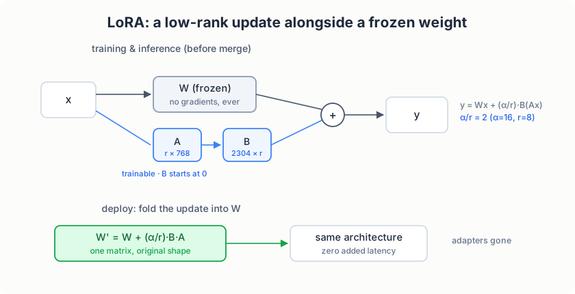
The paper’s two initialization rules
One detail makes LoRA workable, and it is worth slowing down for. At initialization the wrapped layer must compute exactly what the base computed, or the first training step starts by wrecking the base model’s function. The paper’s init guarantees that: B starts at zero, so B @ A = 0 regardless of A, and the wrapped forward is
y = W x + (alpha / r) * B (A x) = W x
bit for bit. A gets kaiming-uniform values (nn.Linear’s default reset);
its distribution only shapes the early gradient path, never the initial
function. test_model.py runs the wrapped and unwrapped models on the
same batch at init and asserts torch.equal.
The second rule is freezing, not just the targets. Every original
parameter gets requires_grad = False before wrapping, and only the
fresh adapters default back to trainable. A first draft of this project
got that wrong (the freeze covered only the wrapped matrices), and the
trainable-count test caught it: “only the adapters train” is an assertion
here, not a hope.
The code
The layer
lora.py replaces an nn.Linear in place with matching parameter names,
so a wrapped model loads the base checkpoint’s tensors without any key
translation, and its own checkpoints stay five-key compatible:
self.weight = nn.Parameter(base.weight.data.clone(), requires_grad=False)
self.lora_A = nn.Parameter(torch.empty(r, base.in_features))
self.lora_B = nn.Parameter(torch.zeros(base.out_features, r))
nn.init.kaiming_uniform_(self.lora_A, a=math.sqrt(5))
# lora_B stays zero: dW = B @ A = 0 at init, so the first forward
# is bit-identical to the base model (Hu et al., 2021, section 4.1)
The forward is the frozen path plus the scaled adapter path; a merged
flag switches the adapter off after folding:
def forward(self, x):
    out = F.linear(x, self.weight)
    if not self.merged:
        lora = F.linear(F.linear(x, self.lora_A), self.lora_B)
        out = out + self.scaling * lora
    return out
Wrapping the model
apply_lora() freezes everything, then suffix-matches module names. Our
c_attn is one fused matrix for Q, K, and V, so the paper’s default
targets (W_q, W_v) are strictly a subset of what it adapts:
for parameter in model.parameters():
    parameter.requires_grad = False
replaced = []
for name, module in list(model.named_modules()):
    if isinstance(module, nn.Linear) and any(
        name.endswith(t) for t in targets
    ):
        parent_name, _, leaf = name.rpartition(".")
        parent = model.get_submodule(parent_name) if parent_name else model
        setattr(parent, leaf, LoRALinear(module, r=r, alpha=alpha))
        replaced.append(name)
The training loop’s only real change
The loop is project 5’s, verbatim, except for what the optimizer sees:
model, arch = load_base_model(args.base_checkpoint, config.DEVICE)
lora_cfg = {"r": config.LORA_R, "alpha": config.LORA_ALPHA,
            "targets": list(config.LORA_TARGETS)}
apply_lora_to(model)
optimizer = configure_optimizer(model)
apply_lora_to does the freeze-then-wrap and prints the trainable
report; configure_optimizer passes only adapter parameters to AdamW, so
the moment buffers shrink from ~1.0 GB to ~3.1 MB and the frozen matrices
never allocate gradient slots. Gradient clipping also runs over the
trainable set only. Data, loss masking, schedule shape, and checkpoint
format are project 5’s, on purpose: the chapter 6 vs chapter 7 loss
curves are measured on identical arrays.
Merging at deploy
The adapter adds one matrix multiply per wrapped module at inference. The paper’s deploy trick removes it: fold the update into the frozen weight and discard the path.
@torch.no_grad()
def merge(self) -> None:
    if self.merged:
        return
    self.weight.data += self.scaling * (self.lora_B @ self.lora_A)
    self.merged = True
The merged layer is a single matrix of the original shape, so the
deployed model is architecturally indistinguishable from the base.
Mathematically (alpha/r) B (A x) = ((alpha/r) B A) x exactly; in floats
the reassociation costs a rounding error, and test_model.py asserts the
merged outputs match the adapter outputs to 1e-6.
What adapters cannot do
An honest limit, measured during development rather than taken on faith: adapter-only training on a RANDOM tiny base barely moves the loss (4.82 to 4.20 on the overfit test, stable across target sets and learning rates). A random frozen base supplies noise features, and a rank-8 correction cannot route through them. LoRA’s premise is that the base is pre-trained and structured; the method tunes a competent model, it does not rescue an incompetent one. The same arithmetic explains the rank sensitivity the paper reports: r is a capacity knob that only matters when the base gives the capacity something to steer.
Running it
# data comes from project 5 (encode once, reuse everywhere)
uv run python phase2_finetuning/project5_sft/prepare_data.py
uv run python phase2_finetuning/project6_lora/test_model.py
uv run python phase2_finetuning/project6_lora/train.py
uv run python phase2_finetuning/project6_lora/generate.py --instruction "Give three tips for staying healthy."
test_model.py runs 8 tests: the init identity, freeze plus
trainable-count arithmetic, target validation, merge equivalence, the
adapter-only overfit, checkpoint round-trips (LoRA and plain checkpoints
both load through generate.load_model), the real base checkpoint wrap,
and the <EOS>-stop sampler contract.
Results
Defaults: r = 8, alpha = 16, targets c_attn, base = project 4 checkpoint, the same 50,973-example Alpaca arrays chapter 6 trained on, 2,400 steps, lr 1e-4, response-only loss.
| Metric | Value |
|---|---|
| Wall time | ~78 min (bf16, ~2.0 s/step incl. eval + snapshot writes) |
| GPU memory | ~4.0 GB of 8 GB |
| Val loss (response tokens), step 0 | 4.9941 (the base model’s number) |
| Val loss after 100 / 400 / 800 steps | 4.478 / 4.070 / 3.927 |
| Final val loss (2,400 steps) | 3.802 (perplexity 44.8) |
| Best checkpoint | final step; val monotone down, no overfit in 3 epochs |
The step-0 number doubles as a check. Chapter 6 measured the base model
at 4.994 on these arrays before any training; the wrapped model, with
393,216 fresh parameters attached, scored 4.9941 at iteration 0.
Zero-initialized B plus a frozen base, verified on the real checkpoint as
well as in test_model.py.
Set against chapter 6, which trained every parameter on identical arrays:
| Metric | Full SFT (ch06) | LoRA r = 8 (this chapter) |
|---|---|---|
| Trainable parameters | 126,273,024 | 393,216 (0.310%) |
| Val loss, start → final | 4.994 → 2.766 | 4.994 → 3.802 |
| Loss improvement captured | 2.228 | 1.192 (about 53%) |
| Perplexity (response tokens) | 15.9 | 44.8 |
| Wall time | ~1 h 42 min (~2.5 s/step) | ~78 min (~2.0 s/step) |
| GPU memory | ~5.8 GB | ~4.0 GB |
LoRA was also the cheaper run per step. The forward pass is unchanged (the adapter path adds one small matmul per block), but the frozen matrices never materialize weight gradients, and the optimizer step plus gradient clip touch 393k parameters instead of 126M. Memory drops for the same reason: no gradient slots or AdamW moments for the frozen 126M.
One caveat on the deploy story: model_final.pt here stores the full
wrapped model (~510 MB), five-key compatible like every other checkpoint
in this repo. The adapter tensors alone are 393,216 × 4 bytes ≈ 1.6 MB;
storing those with a base-checkpoint path would make the per-task
shipping claim from the intro literal.
The same three prompts chapter 6 sampled, after the LoRA run (temperature 0.7):
Q: Give three tips for staying healthy. A: 1. Heathft, 2. Take your healthme, 2. Say your healthme, 2. Say your healthme, 9. Say your healthme, 9. Say your healthme, …
Q: What is the capital of France? A: The capital of France? is the capital of France: The capital of France: The capital of France: A place of its own is the governor of France: A place of the governor of France: A place of the governor of France: …
Q: Rewrite this sentence in past tense: ‘She walks to school.’ A: She walks to school.
The loss table and the samples agree. The adapter captured about half of what full fine-tuning captured (1.19 of the 2.23 loss improvement), and the samples show what half means: it moved toward the response format (numbered lists, answer-shaped openings) without escaping the base model’s repetition attractors. Chapter 6’s model looped too, but over plausible sentences; this one loops over five-word fragments. Full fine-tuning can rewrite the fluency machinery because it edits all 126M parameters; a rank-8 correction on 16 attention projections can only steer it. This is the random-base lesson from the overfit test above, one notch milder: the low-rank assumption recovers what the frozen base can express, and our base (val perplexity 30 on its own corpus, 131M pre-training tokens) is only partly the competent model the paper’s GPT-3 experiments assumed. The missing competence is exactly what adapters cannot supply.
Code tour
| File | What to read |
|---|---|
config.py | LoRA hyperparameters with paper references; the reuse-project-5-data note |
lora.py | LoRALinear, apply_lora() (freeze + wrap), merge() |
model.py | Same GPT as projects 4/5; adapters wrap it at runtime |
train.py | Base load, freeze + wrap, adapter-only optimizer, checkpoints |
generate.py | Loads LoRA and plain checkpoints; <EOS>-stop sampling |
test_model.py | Init identity, freeze/count, merge equivalence, round-trip, base wrap |
Exercises
- Sweep the rank:
--lora_r 1and--lora_r 32against the r = 8 run, same steps. The paper claims low-rank updates generalize even at r = 1; does 126M-parameter GPT agree? - Widen the targets to every Linear (
c_attn,c_proj,fc). Trainable count goes up ~4x; what does the val loss say about where the useful adaptation capacity actually is? - Continued adaptation: start from project 5’s
model_final.ptinstead of the base. Compare against starting from the base and against chapter 6’s full fine-tune. - Measure optimizer-state memory before and after
apply_lorawithtorch.cuda.memory_allocated(). Compare with the table above. - Merge, then sample: run
generate.pyon a merged checkpoint and confirm the outputs are distributionally the same as the unmerged model’s. What could break the equivalence at bf16?
What’s next
SFT (chapter 6) and LoRA (this chapter) teach a model to answer by imitating answers. DPO (project 7) goes one stage further down the alignment recipe: with a prompt and two candidate responses, one preferred, it shifts probability mass toward the preferred one directly, no reward model required. It needs a model that already follows the format, which is exactly what the last two chapters produced.
The Roadmap: 10 Phases, 32 Projects
The full curriculum, from a character-level GPT to a deployed LLM application. Chapters written so far are linked; the rest follow the same pattern as the repository grows.
Phase 1 — Foundation (Part I of this book)
| Project | Topic | Status |
|---|---|---|
| 1 | Character-Level GPT | ✅ Chapter 1 |
| 2 | BPE Tokenizer | ✅ Chapter 2 |
| 3 | Contextual Embeddings (BERT-style) | ✅ Chapter 3 |
| 3B | SimCSE (Sentence Embeddings) | ✅ Chapter 4 |
| 4 | Pre-train 125M Model | ✅ Chapter 5 |
Focus: multi-head attention, transformer blocks, training loops, text generation, masked language modeling, contrastive learning.
Phase 2 — Fine-Tuning
| Project | Topic | Status |
|---|---|---|
| 5 | Supervised Fine-Tuning (SFT) | ✅ Chapter 6 |
| 6 | LoRA Fine-Tuning | ✅ Chapter 7 |
| 7 | DPO (Direct Preference Optimization) |
Focus: instruction formatting, memory-efficient training, preference alignment.
Phase 3 — Core Inference Optimizations
| Project | Topic | Speedup |
|---|---|---|
| 8 | Mixed Precision Training & Inference | 2–4× |
| 9 | KV-Cache | 10–30× |
| 10 | Flash Attention | 2–4× |
Papers: Micikevicius 2018 · Transformer-XL · Flash Attention 1 & 2
Phase 4 — Advanced Inference Optimizations
| Project | Topic | Speedup |
|---|---|---|
| 11 | Prompt Caching | 5–50× |
| 12 | Speculative Decoding | 2–3× |
| 13 | Dynamic Batching | 3–10× |
| 14 | Paged Attention | Near-zero memory waste |
Papers: SemCache · vLLM · Orca · Speculative Sampling
Phase 5 — Quantization
| Project | Topic | Benefit |
|---|---|---|
| 15 | Post-Training Quantization (PTQ) | 2–4× smaller |
| 16 | KV-Cache Quantization | 50% cache reduction |
| 17 | Quantization-Aware Training (QAT) | Better accuracy |
Papers: GPTQ · LLM.int8() · QAT (Jacob 2018)
Phase 6 — Model Compression
| Project | Topic | Reduction |
|---|---|---|
| 18 | Pruning (Structured & Unstructured) | 30–60% |
| 19 | Knowledge Distillation | Smaller models |
| 20 | Weight Sharing | 10–30% |
Papers: Wanda · Distilling Knowledge · ALBERT
Phase 7 — Advanced Architectures
| Project | Topic | Complexity |
|---|---|---|
| 21 | Sparse Attention | O(n√n) |
| 22 | Mixture-of-Experts (MoE) | Same compute, more params |
| 23 | Memory-Efficient Attention | 2–4× less memory |
Papers: Longformer · BigBird · Switch Transformers · Mixtral
Phase 8 — Parallelism & Scaling
| Project | Topic | Outcome |
|---|---|---|
| 24 | Tensor Parallelism | Multi-GPU training |
| 25 | Pipeline Parallelism | Better GPU utilization |
Papers: Megatron-LM · GPipe · PipeDream
Phase 9 — Compiler Optimizations
| Project | Topic | Speedup |
|---|---|---|
| 26 | Operator Fusion | 20–40% |
| 27 | Graph Optimization | 1.5–3× |
| 28 | Early Exit | 30–50% |
Papers: Triton · XLA · TVM · PABEE
Phase 10 — Production Deployment
| Project | Topic | Outcome |
|---|---|---|
| 29 | Model Serving Optimization | Production API |
| 30 | Docker Deployment | One-command deploy |
| 31 | Interactive UI (Gradio) | User-friendly |
The learning pathway
| Phases | Theme |
|---|---|
| 1–2 | Build and fine-tune LLMs |
| 3–4 | Speed up generation |
| 5–6 | Shrink models |
| 7–8 | Train larger models |
| 9–10 | Ship to production |
Projects are cumulative: the tokenizer of Phase 1 feeds the pre-training of Project 4, the model of Project 4 is what gets fine-tuned in Phase 2, and the same model is the one optimized in Phases 3–9. Skipping foundations catches up with you by Phase 3.
Results Log
Measured results from real runs in this repository. Hardware: NVIDIA GeForce RTX 3050 (8 GB), PyTorch 2.11 + CUDA 12.8. Models and datasets are deliberately small so every number is reproducible on a laptop GPU.
Chapter 1 — Character-Level GPT
| Metric | Value |
|---|---|
| Dataset | Tiny Shakespeare (~1M chars) |
| Vocabulary | ~65 characters |
| Model size | ~10M parameters |
| Training time | < 1 hour on GPU |
| Target validation loss | 1.5–1.8 |
Chapter 2 — BPE Tokenizer
| Metric | Value |
|---|---|
| Corpus | WikiText-2 (~11 MB) |
| Vocabulary | 5,000 tokens (3,983 learned merges) |
| Training time (optimized loop) | ~12 minutes |
| Training time (naive full-rescan loop) | ~5 hours |
| Speedup from distinct-word representation | ~50× |
The optimization: count adjacent pairs over distinct words with multiplicities instead of rescanning the full corpus per merge.
Chapter 3 — BERT-style Encoder
| Metric | Value |
|---|---|
| Corpus | WikiText-2 |
| Model size | 4.8M parameters (6 layers, 256 hidden, 8 heads) |
| Iterations | 10,000 (batch 32, block 128) |
| Training time | ~12 minutes on GPU |
| MLM loss | 4.2 → ~1.4 (train), best val 2.85 |
Chapter 4 — SimCSE
Fine-tuned from the Chapter 3 checkpoint on 100k Wikipedia sentences, batch 64, τ = 0.05, lr 5e-5, max sequence length 32.
| Model | STS-B dev Spearman ↑ |
|---|---|
MLM encoder, raw [CLS] (baseline) | 16.6 |
| SimCSE, 1 epoch | 27.0 |
| SimCSE, 3 epochs (final) | 34.7 |
| SimCSE, 5 epochs | 33.5 |
| Metric | Value |
|---|---|
| Time per epoch | ~26 s |
| Improvement over baseline | +18.1 Spearman |
| Paper reference (BERT-base, 110M params, 10⁶ sentences) | 82.5 |
Evaluation protocol: cosine similarity vs human scores, Spearman rank correlation, dropout OFF, without the training-only MLP head. STS-B test labels are hidden (GLUE leaderboard only), so dev is the reportable split.
Chapter 5 — Pre-Training a 125M GPT
Tokenizer (16,384-token BPE, trained on a seeded 100 MB sample of
wiki.train.raw):
| Metric | Value |
|---|---|
| Vocabulary | 16,384 (2,612 characters + 13,768 merges + 4 special tokens) |
| Tokenizer training time | 113.1 s (incremental trainer) |
| Distinct words in sample | 284,771 |
| Compression (probe sentence) | 4.7 chars/token |
| Trainer equivalence test | 116/116 merges identical to naive rescan |
For comparison, the chapter 2 rescan loop needed ~12 minutes for 3,983 merges on WikiText-2; the incremental trainer did 15,367 merges on the same corpus in 24.9 s.
Encoded corpus (uint16 memmap files):
| Split | Documents | Tokens | <UNK> rate |
|---|---|---|---|
| train | 305,497 | 123,564,629 | 0.005% |
| val | 620 | 257,564 | 0.038% |
| test | 708 | 296,257 | 0.007% |
Training run (4,000 steps × 32,768 tokens/step ≈ 131M tokens, one pass over the train split):
| Metric | Value |
|---|---|
| Wall time | 2 h 36 min (RTX 3050, bf16) |
| Throughput | ~14,100 tokens/s steady |
| GPU memory | 5.8 GB of 8 GB |
| Val loss (iter 0 → best) | 9.83 → 3.385 (iter 3,800) |
| Final val loss | 3.408 (perplexity 30.2) |
| Sample quality | article headings, dated Wikipedia voice, confabulated facts |
Context: GPT-2’s 37.5 perplexity on WikiText-103 is zero-shot (trained on WebText, different tokenizer) and not comparable to this in-domain run. A Chinchilla-optimal token budget for 126M parameters would be ~2.5B tokens, about 19× this run (~50 hours at the measured throughput).
Chapter 6 — Supervised Fine-Tuning
Fine-tuned the Chapter 5 base model on Stanford Alpaca (52,002 triples; 28 dropped for empty outputs; 50,973 train / 1,000 val after encoding and a seeded split), Alpaca template, response-only loss masking, lr 2e-5, 2,400 steps = 153,600 example visits (~3.0 epochs).
| Metric | Value |
|---|---|
| Encoding speed | ~1,600 examples/s (~33 s for the full set) |
| Corpus averages | 65.8 prompt + 70.3 response tokens; 0.003% <UNK> |
| Wall time | ~1 h 42 min (bf16, 8 × 8 × 511 batch shape, ~2.5 s/step) |
| GPU memory | ~5.8 GB of 8 GB |
| Val loss (response tokens), base model | 4.994 |
| Val loss, 100 / 400 / 800 steps | 3.708 / 3.168 / 2.954 |
| Final val loss (2,400 steps) | 2.766 (perplexity 15.9) |
| Best checkpoint | iter 2,300 (val 2.769); val monotone down, no overfit in 3 epochs |
| Behavior change | answers in the template slot and stops via <EOS>; facts confabulated, shallow transformations (copied input on a past-tense rewrite) |
Before SFT, the base model continued the template into WikiText prose (“…### Response:= = = = Contents of the House = = = =…”). After SFT it produces answer-shaped spans and ends its turn; sample quality limits are recorded honestly in the chapter.
Chapter 7 — LoRA Fine-Tuning
Adapted the Chapter 5 base model with LoRA (r = 8, alpha = 16, targets:
the fused QKV c_attn in all 16 blocks) on the same encoded Alpaca
arrays as Chapter 6, lr 1e-4, 2,400 steps = 153,600 example visits
(~3.0 epochs), response-only loss.
| Metric | Value |
|---|---|
| Trainable parameters | 393,216 of 126,666,240 (0.310%) |
| Init identity check | iter-0 val loss 4.9941 = the base model’s number |
| Wall time | ~78 min (bf16, ~2.0 s/step) |
| GPU memory | ~4.0 GB of 8 GB (full fine-tune: ~5.8 GB) |
| Final val loss (2,400 steps) | 3.802 (perplexity 44.8) |
| Head-to-head vs Chapter 6 | 4.994 → 2.766 (full) vs 4.994 → 3.802 (LoRA); ~53% of the loss improvement with 0.31% of the parameters |
| Val curve | monotone down, no overfit in 3 epochs |
| Sample behavior | format partially learned; repetition loops over short fragments (full SFT looped over plausible sentences) |
Reproducing
Every number above comes from the commands in
Getting Set Up with default configurations. Checkpoints are
written to checkpoints/ (gitignored); training logs are deterministic
modulo CUDA nondeterminism.