Low-Rank Adaptation (LoRA)
Project source:
phase2_finetuning/project6_lora/Papers: “LoRA: Low-Rank Adaptation of Large Language Models” (Hu et al., 2021) · “Training Language Models to Follow Instructions with Human Feedback” (Ouyang et al., 2022, InstructGPT) · “Stanford Alpaca” (Taori et al., 2023) · “Language Models are Few-Shot Learners” (Brown et al., 2020, GPT-3)
The full fine-tune is the expensive part
Chapter 6 taught the base model to answer instructions by updating all 126,273,024 parameters. The updated weights were the point, but they were also the cost. AdamW keeps two fp32 moment buffers per trainable parameter, so the optimizer state alone is ~2x the model, about a gigabyte here. And every task you adapt for needs its own full weight copy: instruction-following, then summarization, then code, each 500 MB of deltas to store and ship.
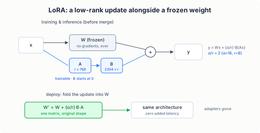
LoRA (Hu et al., 2021) starts from an empirical observation about what full fine-tuning actually does: the change in the weights, dW, has a low intrinsic rank for adaptation tasks. The task-specific adjustments live in a small subspace of the weight space. So make that assumption structural: do not learn dW directly, learn a factorization
dW = B @ A, A is r x k, B is d x r, r << min(d, k)
and run the layer as
y = W x + (alpha / r) * B (A x)
with W frozen. The trainable count per adapted matrix drops from d x k to r x (d + k). On GPT-3, the paper matches full fine-tuning quality with 10,000x fewer trainable parameters, which is the result the method is named for.
The numbers at our scale, with the paper’s rank r = 8 and scale
alpha = 16, adapting the fused QKV projection c_attn (768 -> 2304) in
every one of the 16 blocks:
| Component | Full fine-tune (ch06) | LoRA (this chapter) |
|---|---|---|
| Trainable parameters | 126,273,024 | 393,216 (0.310%) |
| AdamW optimizer state | ~1.0 GB | ~3.1 MB |
| Per-matrix cost | 768 x 2304 = 1.77M | 8 x (768 + 2304) = 24,576 |
| Adapted matrices | all | 16 x c_attn |
Per matrix, the update compresses 72x: 1.77M numbers become 24,576. Sixteen
wrapped modules gives 393,216 trainable parameters, and
test_model.py asserts that exact count so the table stays honest.
The paper’s two initialization rules
One detail makes LoRA workable, and it is worth slowing down for. At initialization the wrapped layer must compute exactly what the base computed, or the first training step starts by wrecking the base model’s function. The paper’s init guarantees that: B starts at zero, so B @ A = 0 regardless of A, and the wrapped forward is
y = W x + (alpha / r) * B (A x) = W x
bit for bit. A gets kaiming-uniform values (nn.Linear’s default reset);
its distribution only shapes the early gradient path, never the initial
function. test_model.py runs the wrapped and unwrapped models on the
same batch at init and asserts torch.equal.
The second rule is freezing, not just the targets. Every original
parameter gets requires_grad = False before wrapping, and only the
fresh adapters default back to trainable. A first draft of this project
got that wrong (the freeze covered only the wrapped matrices), and the
trainable-count test caught it: “only the adapters train” is an assertion
here, not a hope.
The code
The layer
lora.py replaces an nn.Linear in place with matching parameter names,
so a wrapped model loads the base checkpoint’s tensors without any key
translation, and its own checkpoints stay five-key compatible:
self.weight = nn.Parameter(base.weight.data.clone(), requires_grad=False)
self.lora_A = nn.Parameter(torch.empty(r, base.in_features))
self.lora_B = nn.Parameter(torch.zeros(base.out_features, r))
nn.init.kaiming_uniform_(self.lora_A, a=math.sqrt(5))
# lora_B stays zero: dW = B @ A = 0 at init, so the first forward
# is bit-identical to the base model (Hu et al., 2021, section 4.1)
The forward is the frozen path plus the scaled adapter path; a merged
flag switches the adapter off after folding:
def forward(self, x):
    out = F.linear(x, self.weight)
    if not self.merged:
        lora = F.linear(F.linear(x, self.lora_A), self.lora_B)
        out = out + self.scaling * lora
    return out
Wrapping the model
apply_lora() freezes everything, then suffix-matches module names. Our
c_attn is one fused matrix for Q, K, and V, so the paper’s default
targets (W_q, W_v) are strictly a subset of what it adapts:
for parameter in model.parameters():
    parameter.requires_grad = False
replaced = []
for name, module in list(model.named_modules()):
    if isinstance(module, nn.Linear) and any(
        name.endswith(t) for t in targets
    ):
        parent_name, _, leaf = name.rpartition(".")
        parent = model.get_submodule(parent_name) if parent_name else model
        setattr(parent, leaf, LoRALinear(module, r=r, alpha=alpha))
        replaced.append(name)
The training loop’s only real change
The loop is project 5’s, verbatim, except for what the optimizer sees:
model, arch = load_base_model(args.base_checkpoint, config.DEVICE)
lora_cfg = {"r": config.LORA_R, "alpha": config.LORA_ALPHA,
            "targets": list(config.LORA_TARGETS)}
apply_lora_to(model)
optimizer = configure_optimizer(model)
apply_lora_to does the freeze-then-wrap and prints the trainable
report; configure_optimizer passes only adapter parameters to AdamW, so
the moment buffers shrink from ~1.0 GB to ~3.1 MB and the frozen matrices
never allocate gradient slots. Gradient clipping also runs over the
trainable set only. Data, loss masking, schedule shape, and checkpoint
format are project 5’s, on purpose: the chapter 6 vs chapter 7 loss
curves are measured on identical arrays.
Merging at deploy
The adapter adds one matrix multiply per wrapped module at inference. The paper’s deploy trick removes it: fold the update into the frozen weight and discard the path.
@torch.no_grad()
def merge(self) -> None:
    if self.merged:
        return
    self.weight.data += self.scaling * (self.lora_B @ self.lora_A)
    self.merged = True
The merged layer is a single matrix of the original shape, so the
deployed model is architecturally indistinguishable from the base.
Mathematically (alpha/r) B (A x) = ((alpha/r) B A) x exactly; in floats
the reassociation costs a rounding error, and test_model.py asserts the
merged outputs match the adapter outputs to 1e-6.
What adapters cannot do
An honest limit, measured during development rather than taken on faith: adapter-only training on a RANDOM tiny base barely moves the loss (4.82 to 4.20 on the overfit test, stable across target sets and learning rates). A random frozen base supplies noise features, and a rank-8 correction cannot route through them. LoRA’s premise is that the base is pre-trained and structured; the method tunes a competent model, it does not rescue an incompetent one. The same arithmetic explains the rank sensitivity the paper reports: r is a capacity knob that only matters when the base gives the capacity something to steer.
Running it
# data comes from project 5 (encode once, reuse everywhere)
uv run python phase2_finetuning/project5_sft/prepare_data.py
uv run python phase2_finetuning/project6_lora/test_model.py
uv run python phase2_finetuning/project6_lora/train.py
uv run python phase2_finetuning/project6_lora/generate.py --instruction "Give three tips for staying healthy."
test_model.py runs 8 tests: the init identity, freeze plus
trainable-count arithmetic, target validation, merge equivalence, the
adapter-only overfit, checkpoint round-trips (LoRA and plain checkpoints
both load through generate.load_model), the real base checkpoint wrap,
and the <EOS>-stop sampler contract.
Results
Defaults: r = 8, alpha = 16, targets c_attn, base = project 4 checkpoint, the same 50,973-example Alpaca arrays chapter 6 trained on, 2,400 steps, lr 1e-4, response-only loss.
| Metric | Value |
|---|---|
| Wall time | ~78 min (bf16, ~2.0 s/step incl. eval + snapshot writes) |
| GPU memory | ~4.0 GB of 8 GB |
| Val loss (response tokens), step 0 | 4.9941 (the base model’s number) |
| Val loss after 100 / 400 / 800 steps | 4.478 / 4.070 / 3.927 |
| Final val loss (2,400 steps) | 3.802 (perplexity 44.8) |
| Best checkpoint | final step; val monotone down, no overfit in 3 epochs |
The step-0 number doubles as a check. Chapter 6 measured the base model
at 4.994 on these arrays before any training; the wrapped model, with
393,216 fresh parameters attached, scored 4.9941 at iteration 0.
Zero-initialized B plus a frozen base, verified on the real checkpoint as
well as in test_model.py.
Set against chapter 6, which trained every parameter on identical arrays:
| Metric | Full SFT (ch06) | LoRA r = 8 (this chapter) |
|---|---|---|
| Trainable parameters | 126,273,024 | 393,216 (0.310%) |
| Val loss, start → final | 4.994 → 2.766 | 4.994 → 3.802 |
| Loss improvement captured | 2.228 | 1.192 (about 53%) |
| Perplexity (response tokens) | 15.9 | 44.8 |
| Wall time | ~1 h 42 min (~2.5 s/step) | ~78 min (~2.0 s/step) |
| GPU memory | ~5.8 GB | ~4.0 GB |
LoRA was also the cheaper run per step. The forward pass is unchanged (the adapter path adds one small matmul per block), but the frozen matrices never materialize weight gradients, and the optimizer step plus gradient clip touch 393k parameters instead of 126M. Memory drops for the same reason: no gradient slots or AdamW moments for the frozen 126M.
One caveat on the deploy story: model_final.pt here stores the full
wrapped model (~510 MB), five-key compatible like every other checkpoint
in this repo. The adapter tensors alone are 393,216 × 4 bytes ≈ 1.6 MB;
storing those with a base-checkpoint path would make the per-task
shipping claim from the intro literal.
The same three prompts chapter 6 sampled, after the LoRA run (temperature 0.7):
Q: Give three tips for staying healthy. A: 1. Heathft, 2. Take your healthme, 2. Say your healthme, 2. Say your healthme, 9. Say your healthme, 9. Say your healthme, …
Q: What is the capital of France? A: The capital of France? is the capital of France: The capital of France: The capital of France: A place of its own is the governor of France: A place of the governor of France: A place of the governor of France: …
Q: Rewrite this sentence in past tense: ‘She walks to school.’ A: She walks to school.
The loss table and the samples agree. The adapter captured about half of what full fine-tuning captured (1.19 of the 2.23 loss improvement), and the samples show what half means: it moved toward the response format (numbered lists, answer-shaped openings) without escaping the base model’s repetition attractors. Chapter 6’s model looped too, but over plausible sentences; this one loops over five-word fragments. Full fine-tuning can rewrite the fluency machinery because it edits all 126M parameters; a rank-8 correction on 16 attention projections can only steer it. This is the random-base lesson from the overfit test above, one notch milder: the low-rank assumption recovers what the frozen base can express, and our base (val perplexity 30 on its own corpus, 131M pre-training tokens) is only partly the competent model the paper’s GPT-3 experiments assumed. The missing competence is exactly what adapters cannot supply.
Code tour
| File | What to read |
|---|---|
config.py | LoRA hyperparameters with paper references; the reuse-project-5-data note |
lora.py | LoRALinear, apply_lora() (freeze + wrap), merge() |
model.py | Same GPT as projects 4/5; adapters wrap it at runtime |
train.py | Base load, freeze + wrap, adapter-only optimizer, checkpoints |
generate.py | Loads LoRA and plain checkpoints; <EOS>-stop sampling |
test_model.py | Init identity, freeze/count, merge equivalence, round-trip, base wrap |
Exercises
- Sweep the rank:
--lora_r 1and--lora_r 32against the r = 8 run, same steps. The paper claims low-rank updates generalize even at r = 1; does 126M-parameter GPT agree? - Widen the targets to every Linear (
c_attn,c_proj,fc). Trainable count goes up ~4x; what does the val loss say about where the useful adaptation capacity actually is? - Continued adaptation: start from project 5’s
model_final.ptinstead of the base. Compare against starting from the base and against chapter 6’s full fine-tune. - Measure optimizer-state memory before and after
apply_lorawithtorch.cuda.memory_allocated(). Compare with the table above. - Merge, then sample: run
generate.pyon a merged checkpoint and confirm the outputs are distributionally the same as the unmerged model’s. What could break the equivalence at bf16?
What’s next
SFT (chapter 6) and LoRA (this chapter) teach a model to answer by imitating answers. DPO (project 7) goes one stage further down the alignment recipe: with a prompt and two candidate responses, one preferred, it shifts probability mass toward the preferred one directly, no reward model required. It needs a model that already follows the format, which is exactly what the last two chapters produced.