SimCSE: Sentence Embeddings
Project source:
phase1_foundation/project3b_simcse/Papers: “SimCSE: Simple Contrastive Learning of Sentence Embeddings” (Gao, Yao & Chen, EMNLP 2021) · “Understanding Contrastive Representation Learning through Alignment and Uniformity on the Hypersphere” (Wang & Isola, 2020) · STS-B (Cer et al., 2017)
The problem
Chapter 3’s encoder produces contextual token embeddings. Downstream tasks (semantic search, clustering, duplicate detection) need a single vector per sentence where similar sentences end up close together. Averaging the encoder’s outputs doesn’t give you that geometry.
SimCSE fixes it with an almost absurdly simple recipe:
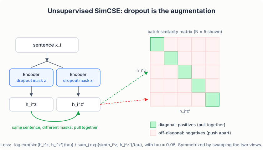
Feed the same sentence into the encoder twice. Because dropout masks are sampled independently, you get two slightly different embeddings. Train the encoder to pull those two together and push every other sentence in the batch away.
No paraphrase data, no translation pairs. Dropout is the data augmentation. The paper puts it plainly:
“dropout acts as minimal data augmentation, and removing it leads to a representation collapse.”
The objective
For a mini-batch of N sentences (equation 4 of the paper):
                  exp(sim(h_i^z, h_i^z')/τ)
l_i = -log -------------------------------------------
           Σ_j exp(sim(h_i^z, h_j^z')/τ)
| Symbol | Meaning |
|---|---|
h_i^z | Embedding of sentence x_i under dropout mask z |
h_i^z' | The same sentence under an independent mask z' |
sim(·,·) | Cosine similarity |
τ | Temperature, 0.05 for unsupervised SimCSE |
This is an N-way classification over the batch: each row of the similarity matrix must find its own positive on the diagonal. The loss is symmetrized by swapping the two views.
Why it works: alignment and uniformity
Wang & Isola (2020) characterize good contrastive spaces with two metrics
(both implemented in model.py):
- Alignment: similar sentences map to nearby points (positives are close)
- Uniformity: embeddings spread evenly over the hypersphere
The paper’s diagnostic: models with no dropout, or with a fixed dropout mask shared by both copies, trivially make the two views identical. Their alignment collapses to zero but their representations clump, so uniformity is destroyed and STS-B degrades dramatically. Independent dropout masks keep alignment steady while still improving uniformity. Starting from a pre-trained checkpoint matters too: “it provides good initial alignment.”
The “MLP trick”
During training, a one-layer MLP with tanh sits on top of the [CLS]
embedding, and the contrastive pressure flows through it. At evaluation
the head is discarded and the raw [CLS] embedding is used, which is worth
1–2 Spearman points. The intuition: let the loss shape the space through a
disposable projection, leaving the underlying embedding closer to its
pre-trained manifold.
The code
This is the repository’s code
(model.py,
train.py,
evaluate.py)
with the commentary docstrings trimmed. Excerpts are condensed and lightly
reformatted; the logic matches the repository.
Equation 4, in code
def simcse_loss(z1, z2, temperature):
    # PAPER: SimCSE, Gao et al. (2021), equation 4
    z1 = F.normalize(z1, p=2, dim=-1)      # L2-normalize: dot product == cosine
    z2 = F.normalize(z2, p=2, dim=-1)

    sim_12 = z1 @ z2.t() / temperature     # (N, N) scaled cosine similarities
    sim_21 = z2 @ z1.t() / temperature     # the same matrix, views swapped

    labels = torch.arange(z1.size(0), device=z1.device)  # positive of row i is column i

    loss_12 = F.cross_entropy(sim_12, labels)
    loss_21 = F.cross_entropy(sim_21, labels)
    return (loss_12 + loss_21) / 2
Map each line onto the formula from the objective section. Normalizing
both views to unit length turns the dot product into cosine similarity.
z1 @ z2.t() builds the whole batch similarity matrix at once; dividing
by τ = 0.05 stretches it twenty-fold, which is what makes off-diagonal
negatives hard (their similarities differ by fractions, but after
scaling those fractions are the entire game). The labels are the identity:
row i must pick out column i, its own re-encoding. And because
F.cross_entropy computes -log softmax over each row, the denominator
of equation 4, the sum over all j, is exactly what softmax normalizes
against. The symmetrization at the end trains both directions.
The two forward passes
            # Two forward passes = two independent dropout masks (the
            # entire "augmentation" of unsupervised SimCSE)
            z1 = encoder.encode(idx, attention_mask, project=config.USE_MLP_HEAD)
            z2 = encoder.encode(idx, attention_mask, project=config.USE_MLP_HEAD)

            loss = simcse_loss(z1, z2, config.TEMPERATURE)
Earlier in the same function there is encoder.train() # dropout ON - it IS the augmentation. That comment is the whole method: same batch, same
tokens, no other transformation, two calls. Every stochastic layer inside
the encoder (attention dropout, residual dropout, embedding dropout)
resamples its mask independently on each call, and the gap between the two
embeddings is the positive pair the loss pulls together. If the encoder is
put in eval mode, both calls return the identical tensor, the loss is
log(N), and nothing is learned.
The MLP head and pooling
class MLPHead(nn.Module):
    # PAPER: Gao et al. (2021): "an MLP layer (with one tanh activation) on
    # top of the [CLS] representation ... used only for training but not
    # for evaluation"
    def __init__(self, n_embd):
        super().__init__()
        self.dense = nn.Linear(n_embd, n_embd)
        self.activation = nn.Tanh()

    def forward(self, cls_hidden):
        return self.activation(self.dense(cls_hidden))
        if self.pooler == "cls":
            emb = hidden[:, 0, :]              # the [CLS] hidden state
        elif self.pooler == "mean":
            mask = attention_mask.unsqueeze(-1).float()
            emb = (hidden * mask).sum(dim=1) / mask.sum(dim=1).clamp(min=1.0)
        else:
            raise ValueError(f"Unknown pooler: {self.pooler}")

        if project:                            # training only: the MLP trick
            emb = self.mlp_head(emb)
        return emb
The project flag is where the train/eval asymmetry lives: training
passes route the contrastive pressure through the disposable projection,
evaluation calls encode(..., project=False) and uses the raw [CLS]
embedding. Mean pooling exists as the comparison baseline; it excludes
[PAD] positions via the attention mask so padding cannot dilute the
average.
Alignment and uniformity
def alignment_and_uniformity(z1, z2, temperature=0.05):
    # Wang & Isola (2020); SimCSE Section 3 uses these to explain WHY dropout works
    z1 = F.normalize(z1, p=2, dim=-1)
    z2 = F.normalize(z2, p=2, dim=-1)

    alignment = (z1 - z2).norm(p=2, dim=-1).pow(2).mean().item()

    all_z = torch.cat([z1, z2], dim=0)
    sq_pdist = torch.pdist(all_z, p=2).pow(2)
    uniformity = (-sq_pdist.mul(-2.0 * temperature).exp().mean().log()).item()
    return alignment, uniformity
Both numbers read “lower is better”. Alignment is the mean squared distance between positive pairs; uniformity is a soft measure of how evenly all embeddings spread over the sphere. They are diagnostics, not losses: the collapse the paper warns about shows up as alignment crashing toward zero while uniformity explodes, which is precisely what you observe if you run the exercise with dropout disabled.
The evaluation protocol
@torch.no_grad()
def evaluate_stsb(encoder, split="validation", device=None):
    s1, s2, gold = load_sts_b(split)

    emb1 = encode_sentences(encoder, s1, device=device)   # eval mode: dropout OFF
    emb2 = encode_sentences(encoder, s2, device=device)   # no MLP head either

    e1 = F.normalize(torch.from_numpy(emb1), p=2, dim=-1)
    e2 = F.normalize(torch.from_numpy(emb2), p=2, dim=-1)
    cosine = (e1 * e2).sum(dim=-1).numpy()

    spearman = spearmanr(cosine, gold).statistic
    return float(spearman) * 100
The three contract points from the paper are all visible here. Dropout is
off (encode_sentences calls encoder.eval()), so scores are
reproducible. The MLP head is bypassed. And the reported number is
Spearman, not Pearson: STS-B quality is judged by whether the model’s
ranking of sentence pairs agrees with the human ranking, so what matters
is the correlation between ranks, not raw values.
Evaluation: STS-B
The Semantic Textual Similarity Benchmark (Cer et al., 2017) provides 1,500 dev sentence pairs scored 0–5 by humans. Encode both sentences of every pair (dropout OFF, deterministic), compute cosine similarity, and report the Spearman rank correlation with the human scores. The paper’s BERT-base result: 82.5 dev Spearman.
Note: the GLUE test split’s labels are hidden (leaderboard only), so the dev split is the reportable number.
Results
Trained on 100k Wikipedia sentences, batch 64, τ = 0.05, lr 5e-5, max sequence length 32, on an RTX 3050:
| Model | STS-B dev Spearman |
|---|---|
Project 3 MLM encoder, raw [CLS] (baseline) | 16.6 |
| SimCSE, 1 epoch | 27.0 |
| SimCSE, 3 epochs (final) | 34.7 |
| SimCSE, 5 epochs (overfits) | 33.5 |
That is +18.1 Spearman over the baseline. The paper’s number is higher because their model has 110M parameters and 10⁶ sentences; the pipeline here is theirs, unchanged. Each epoch takes about 26 seconds on the GPU, so hyperparameter experiments are cheap.
Running it
# Sentence corpus + STS-B
uv run python phase1_foundation/project3b_simcse/download_data.py

# Sanity-test the mechanics before training (runs anywhere, seconds)
uv run python phase1_foundation/project3b_simcse/test_model.py

# Train, then evaluate
uv run python phase1_foundation/project3b_simcse/train.py
uv run python phase1_foundation/project3b_simcse/evaluate.py
The sanity tests verify the machinery itself: two forward passes with dropout ON produce different embeddings (if not, the positive pair is degenerate); aligned positives yield lower loss than misaligned ones; gradients reach both the encoder and the MLP head.
Code tour
| File | What to read |
|---|---|
model.py | SimCSEEncoder (wraps Project 3’s BERT), MLPHead, simcse_loss, alignment_and_uniformity |
data.py | Sentence loading, [CLS] s [SEP] [PAD] batching |
train.py | Two-view training loop, warmup + linear decay |
evaluate.py | STS-B protocol |
test_model.py | The sanity suite |
Exercises
- Turn dropout off (
p=0) and retrain. Watch the collapse the paper predicts (Section 3, Table 3). - Swap
[CLS]pooling for mean pooling. Which wins at this scale? - Train on the full extracted corpus (raise
MAX_SENTENCES): does more data close the gap faster than more epochs?
What’s next
Phase 2 applies the same from-scratch discipline to fine-tuning: SFT, LoRA, and DPO. Phase 3 then makes inference fast: mixed precision, KV-cache, and Flash Attention.